Iterative proportional fitting of an abundance table to Hill-N2 marginals

Function for pre-processing/transforming an abundance table by iterative proportional fitting, so that the transformed table has marginals proportional to N2 or N2(1-N2/N) with N the number of elements in the margin. Hill-N2 is the effective number of species. It is of intrinsic interest in weighted averaging (CWM and SNC) as their variance is approximately inversely proportional to N2 (ter Braak 2019), and therefore of interest in dc_CA.

Usage

ipf2N2(
  Y,
  max_iter = 1000,
  updateN2 = TRUE,
  N2N_N2_species = TRUE,
  N2N_N2_sites = FALSE,
  crit = 0.01
)

Arguments

Y: abundance table (matrix or dataframe-like), ideally, with names for rows and columns. BEWARE: all rows and columns should have positive sums!
max_iter: maximum number of iterative proportional fitting (ipf) iterations. If max_iter == 0, the columns are divided by their informativeness (N2) or N2(1-N2/N)) without further pre-processing. The row sums are sums of informativeness instead of effective number of informative species.
updateN2: logical, default TRUE. If FALSE the marginal sums are proportional to the N2-marginals of the initial table, but the N2-marginals of the returned matrix may not be equal to their marginal sum. If updateN2 = TRUE and N2N_N2_species=TRUE (the default), the column marginals are N2(N-N2)/N with N the number of sites. The row sums are then proportional to, what we term, the effective number of informative species. If N2N_N2_species = FALSE, the returned transformed table has N2 columns marginals, i.e. colSums(Y2) = const*N2species(Y2) with Y2 the return value of ipf2N2 and const a constant. If converged, N2 row marginals are equal to the row sums, i.e. rowSums(Y2) = approx. N2sites(Y2).
N2N_N2_species: Set marginals proportional to N2(1-N2/N) Default TRUE.
N2N_N2_sites: Default FALSE. Do not change.
crit: stopping criterion.

Value

a matrix of the same order as the input Y, obtained after ipf to N2-marginals.

Details

Applying ipf2N2 with N2N_N2_species=FALSE to an presence-absence data table returns the same table. However, a species that occurs everywhere (or in most of the sites) is not very informative. This is acknowledged with the default option N2N_N2_species=TRUE. Then, with N2N_N2_species=TRUE, species that occur in more than halve the number of sites are down-weighted, so that the row sum is no longer equal to the richness of the site (the number of species), but proportional to the number of informative species.

References

ter Braak, C.J.F. (2019). New robust weighted averaging- and model-based methods for assessing trait-environment relationships. Methods in Ecology and Evolution, 10 (11), 1962-1971. doi:10.1111/2041-210X.13278

Examples

data("dune_trait_env")

# rownames are carried forward in results
rownames(dune_trait_env$comm) <- dune_trait_env$comm$Sites
Y <- dune_trait_env$comm[, -1] # must delete "Sites"
Y_N2 <- ipf2N2(Y, updateN2 = FALSE, N2N_N2_species = FALSE)
attr(Y_N2, "iter") # 4
#> [1] 4

# show that column margins of the transform matrix are
# equal to the Hill N2 values
diff(range(colSums(Y_N2) / apply(X = Y, MARGIN = 2, FUN = fN2))) #  8.881784e-16
#> [1] 8.881784e-16
diff(range(rowSums(Y_N2) / apply(X = Y, MARGIN = 1, FUN = fN2))) #  0.07077207
#> [1] 0.07077207

Y_N2i <- ipf2N2(Y, updateN2 = TRUE, N2N_N2_species = FALSE)
attr(Y_N2i, "iter") # 5
#> [1] 5
diff(range(colSums(Y_N2i) / apply(X = Y_N2i, MARGIN = 2, FUN = fN2))) # 2.220446e-15
#> [1] 2.220446e-15
diff(range(rowSums(Y_N2i) / apply(X = Y_N2i, MARGIN = 1, FUN = fN2))) # 0.105742
#> [1] 0.105742

# the default version:
Y_N2N_N2i <- ipf2N2(Y)
# ie. 
# Y_N2N_N2i <- ipf2N2(Y, updateN2 = TRUE, N2N_N2_species = TRUE)
attr(Y_N2N_N2i, "iter") # 16
#> [1] 16
N2 <- apply(X = Y_N2N_N2i, MARGIN = 2, FUN = fN2)
N <- nrow(Y)
diff(range(colSums(Y_N2N_N2i) / (N2 * (N - N2)))) # 2.220446e-16
#> [1] 2.220446e-16

N2_sites <- apply(X = Y_N2N_N2i, MARGIN = 1, FUN = fN2)
R <- rowSums(Y_N2N_N2i)
N * max(N2_sites / sum(N2_sites) - R / sum(R)) # 0.009579165
#> [1] 0.009579165

sum(Y_N2N_N2i) - sum(Y)
#> [1] 0

mod0 <- dc_CA(formulaEnv = ~ A1 + Moist + Mag + Use + Manure,
              formulaTraits = ~ SLA + Height + LDMC + Seedmass + Lifespan,
              response = Y,  
              dataEnv = dune_trait_env$envir,
              dataTraits = dune_trait_env$traits, 
              divide = FALSE,
              verbose = FALSE)

mod1 <- dc_CA(formulaEnv = ~ A1 + Moist + Mag + Use + Manure,
              formulaTraits = ~ SLA + Height + LDMC + Seedmass + Lifespan,
              response = Y_N2N_N2i,  
              dataEnv = dune_trait_env$envir,
              dataTraits = dune_trait_env$traits, 
              verbose = FALSE)
#> Argument divideBySiteTotals set to FALSE, as species totals are proportional to N2(N-N2).
#> You can overrule this by specifying divideBySiteTotals explicitly.

mod1$eigenvalues / mod0$eigenvalues
#>     dcCA1     dcCA2     dcCA3     dcCA4     dcCA5 
#> 1.2131999 1.3273601 1.3471699 1.5570817 0.8440445 
# ratios of eigenvalues greater than 1,
# indicate axes with higher (squared) fourth-corner correlation

# ipf2N2 for a presence-absence data matrix                                   
Y_PA <- 1 * (Y > 0)
Y_PA_N2 <- ipf2N2(Y_PA, N2N_N2_species = FALSE)
attr(Y_PA_N2, "iter") # 1
#> [1] 1
diff(range(Y_PA - Y_PA_N2)) # 4.440892e-16, i.e no change
#> [1] 4.440892e-16

Y_PA_N2i <- ipf2N2(Y_PA, N2N_N2_species = TRUE)
attr(Y_PA_N2i, "iter") # 9
#> [1] 9
N_occ <- colSums(Y_PA) # number of occurrences of species
N <- nrow(Y_PA)
plot(N_occ, colSums(Y_PA_N2i))

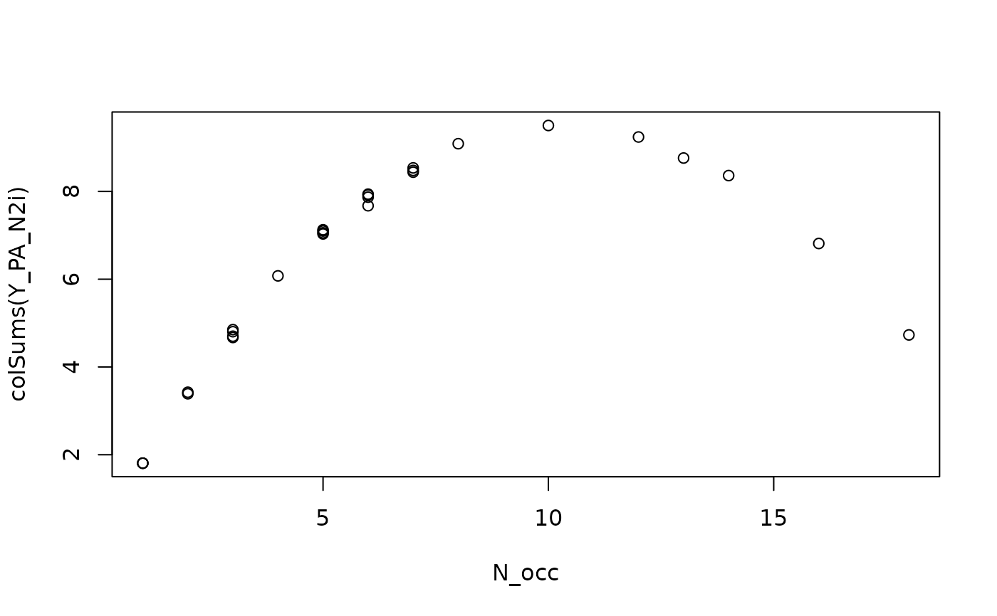cor(colSums(Y_PA_N2i), N_occ * (N - N_occ)) # 0.9916
#> [1] 0.9916937
mod2 <- dc_CA(formulaEnv = ~ A1 + Moist + Mag + Use + Manure,
              formulaTraits = ~ SLA + Height + LDMC + Seedmass + Lifespan,
              response = Y_PA,  
              dataEnv = dune_trait_env$envir,
              dataTraits = dune_trait_env$traits,
              divideBySiteTotals = FALSE,
              verbose = FALSE)
        
mod3 <- dc_CA(formulaEnv = ~ A1 + Moist + Mag + Use + Manure,
              formulaTraits = ~ SLA + Height + LDMC + Seedmass + Lifespan,
              response = Y_PA_N2i,  
              dataEnv = dune_trait_env$envir,
              dataTraits = dune_trait_env$traits,
              verbose = FALSE)
#> Argument divideBySiteTotals set to FALSE, as species totals are proportional to N2(N-N2).
#> You can overrule this by specifying divideBySiteTotals explicitly.
        
mod3$eigenvalues / mod2$eigenvalues
#>    dcCA1    dcCA2    dcCA3    dcCA4    dcCA5 
#> 1.612991 1.320169 1.609431 1.680960 1.311264 
# ratios of eigenvalues greater than 1,
# indicate axes with higher (squared) fourth-corner correlation