Multi-trait GWAS with the statgenQTLxT package

The statgenQTLxT package performs multi-trait and multi-environment Genome Wide Association Studies (GWAS), following the approach of (Zhou and Stephens 2014). It builds on the statgenGWAS package (for single trait GWAS) which is available from CRAN. The package uses data structures and plots defined in the statgenGWAS package. It is recommended to read the vignette of this package, accessible in R via vignette(package = "statgenGWAS") or online at https://biometris.github.io/statgenGWAS/articles/GWAS.html to get a general idea of those.

Multi-Trait GWAS

Theoretical background

Multi-trait GWAS in the statgenQTLxT package estimates and tests the effect of a SNP in different trials or on different traits, one SNP at a time. Genetic and residual covariances are fitted only once, for a model without SNPs. Given balanced data on $n$ genotypes and $p$ traits (or trials) we fit a mixed model of the form

$Y = \left(\begin{array}{c} Y_1 \\ \vdots \\ Y_p\end{array}\right) = \left(\begin{array}{c} X\gamma_1 \\ \vdots \\ X\gamma_p\end{array}\right) + \left(\begin{array}{c} x\beta_1 \\ \vdots \\ x\beta_p\end{array}\right) + \left(\begin{array}{c} G_1 \\ \vdots \\ G_p\end{array}\right) + \left(\begin{array}{c} E_1 \\ \vdots \\ E_p\end{array}\right)$

where $Y_1$ to $Y_p$ are $n × 1$ vectors with the phenotypic values for traits or trials $1, \ldots, p$. $x$ is the $n × 1$ vector of scores for the marker under consideration, and $X$ the $n × q$ design matrix for the other covariates. By default only a trait (environment) specific intercept is included. The vector containing the genetic background effects $G_1, \ldots, G_p$ is Gaussian with zero mean and covariance $V_g \otimes K$, where $V_g$ is a $p × p$ matrix of genetic (co)variances, and $K$ an $n × n$ kinship matrix. Similarly, the residual errors ($E_1, \ldots, E_p$) have covariance $V_e \otimes I_n$, for a $p × p$ matrix $V_e$ of residual (co)variances.

Hypotheses for the SNP-effects

For each SNP, the null-hypothesis $\beta_1 = \dots = \beta_p = 0$ is tested, using the likelihood ratio test (LRT) described in (Zhou and Stephens 2014). If estCom = TRUE, additional tests for a common effect and for QTL-by-trait (QTL × T) or QTL-by-environment (QTL × E) are performed, using the parameterization $\beta_j = \alpha + \alpha_j (1 \leq j \leq p)$. As in (Korte et al. 2012), we use likelihood ratio tests, but not restricted to the bivariate case. For the common effect, we fit the reduced model $\beta_j = \alpha$, and test if $\alpha = 0$. For the interactions, we test if $\alpha_1 = \dots = \alpha_p = 0$.

Models for the genetic and residual covariance

$V_g$ and $V_e$ can be provided by the user (fitVarComp = FALSE); otherwise one of the following models is used, depending on covModel. If covModel = "unst", an unstructured model is assumed, as in (Zhou and Stephens 2014): $V_g$ and $V_e$ can be any positive-definite matrix, requiring a total of $p(p+1)/2$ parameters per matrix. If covModel = "fa", a factor-analytic model is fitted using an EM-algorithm, as in (Millet et al. 2016). $V_g$ and $V_e$ are assumed to be of the form $W W^t + D$, where $W$ is a $p × m$ matrix of factor loadings and $D$ a diagonal matrix with trait or environment specific values. $m$ is the order of the model, and the arguments mG and mE specify the order used for respectively $V_g$ and $V_e$. maxIter sets the maximum number of iterations used in the EM-algorithm. Finally, if covModel = "pw", $V_g$ and $V_e$ are estimated ‘pairwise’, as in (Furlotte and Eskin 2015). Looping over pairs of traits or trials $1 \leq j < k \leq p$, $V_g[j,k] = V_g[k,j]$ and $V_e[j,k] = V_e[k,j]$ are estimated assuming a bivariate mixed model. The diagonals of $V_g$ and $V_e$ are fitted assuming univariate mixed models. If the resulting $V_g$ or $V_e$ is not positive-definite, they are replaced by the nearest positive-definite matrix. In case covModel = "unst" or "pw" it is possible to assume that $V_e$ is diagonal (VeDiag = TRUE).

The class `gData`

Data for analysis on genomic data comes from different sources and is stored in one data object of class gData (genomic Data) for convenience. A gData object will contain all data needed for performing analyses, so the first thing to do when using the statgenQTLxT package is creating a gData object; see the statgenGWAS package for more details. A gData object contains the following components:

Marker map, a data.frame describing the physical positions of the markers on the chromosomes,
Marker matrix, a numerical matrix containing the genotyping,
Phenotypic data, either a single data.frame or a list of data.frames containing the phenotypic data,
Kinship matrix, a matrix describing the genetic relatedness between the different genotypes,
Further covariates that can be used in the analyses.

In our examples below we will show how a gData object is created.

Worked example 1: multiple traits in one trial

As examples of the functionality of the package two worked examples are provided using maize data from the European Union project DROPS. The data is available from https://doi.org/10.15454/IASSTN (Millet et al. 2019) and the relevant data sets are included as data.frames in the statgenGWAS package. We will first show how to load the data and create a gData object. Users already familiar with the statgenGwas packages might want to skip this part and go straight to Running Multi-trait GWAS section.

dropsMarkers contains the coded marker information for 41,722 SNPs and 246 genotypes. dropsMap contains information about the positions of those SNPs on the B73 reference genome V2. dropsPheno contains data for the genotypic means (Best Linear Unbiased Estimators, BLUEs) for a subset of ten experiments, with one value per experiment per genotype, for eight traits. For a more detailed description of the contents of the data see help(dropsData, package = statgenGWAS).

Create gData object

The first step is to create a gData object from the raw data that can be used for the GWAS analysis. For this the raw data has to be converted to a suitable format for a gData object, see help(createGData, package = statgenGWAS) and the statgenGWAS vignette for more details.

When running a multi-trait or multi-environment GWAS, all traits used in the analysis should be in the same data.frame, with genotype as first column and the phenotypic data in subsequent columns. In case of a multi-trait analysis the phenotypic columns contain different traits, measured in one environment, while for a multi-environment the columns correspond to the different environments (same trait). In both cases the data.frame may only contain phenotypic data. Additional covariates need to be stored in covar.

Below are some examples of what these data.frames should look like.

genotype	Trait1	Trait2	Trait3
G1	0.3	17	277
G2	0.4	19	408
G3	0.5	17	206
G4	0.7	13	359

genotype	Trait1-Trial1	Trait1-Trial2	Trait1-Trial3
G1	0.3	0.7	0.5
G2	0.4	0.9	0.1
G3	0.5	0.8	0.2
G4	0.7	0.5	0.4

In our first example, we want to perform multi-trait GWAS for one of the DROPS environments. dropsPheno contains genotypic means for six traits in ten trials. To run a multi-trait GWAS analysis for each of the ten trials, the data has to be added as a list of ten data.frames. Recall that these data.frames should have “genotype” as their first column and may only contain traits after that. Other columns need to be dropped.

The code below creates this list of data.frames from dropsPheno.

data(dropsPheno, package = "statgenGWAS")

## Convert phenotypic data to a list.
colnames(dropsPheno)[1] <- "genotype"
dropsPheno <- dropsPheno[c("Experiment", "genotype", "grain.yield", "grain.number",
                           "anthesis", "silking", "plant.height", "ear.height")]
## Split data by experiment.
dropsPhenoList <- split(x = dropsPheno, f = dropsPheno[["Experiment"]])
## Remove Experiment column.
## phenotypic data should consist only of genotype and traits.
dropsPhenoList <- lapply(X = dropsPhenoList, FUN = `[`, -1)

If the phenotypic data consists of only one trial/experiment, it can be added as a single data.frame without first converting it to a list. In that case createGData will convert the input to a list with one item.

Now a gData object containing map, marker information, and phenotypes can be created. Kinship matrix and covariates may be added later on.

## Load marker data.
data("dropsMarkers", package = "statgenGWAS")
## Add genotypes as row names of dropsMarkers and drop Ind column.
rownames(dropsMarkers) <- dropsMarkers[["Ind"]]
dropsMarkers <- dropsMarkers[, -1]

## Load genetic map.
data("dropsMap", package = "statgenGWAS")
## Add genotypes as row names of dropsMap.
rownames(dropsMap) <- dropsMap[["SNP.names"]]
## Rename Chromosome and Position columns.
colnames(dropsMap)[2:3] <- c("chr", "pos")

## Create a gData object containing map, marker and phenotypic information.
gDataDrops <- statgenGWAS::createGData(geno = dropsMarkers,
                                       map = dropsMap, 
                                       pheno = dropsPhenoList)

To get an idea of the contents of the data a summary of the gData object can be made. This will give an overview of the content of the map and markers and also print a summary per trait per trial. Since there are ten trials and six traits in gDataDrops we restrict the output to one trial, using the trials argument of the summary function.

## Summarize gDataDrops.
summary(gDataDrops, trials = "Mur13W")
#> map
#>  Number of markers: 41722 
#>  Number of chromosomes: 10 
#> 
#> markers
#>  Number of markers: 41722 
#>  Number of genotypes: 246 
#>  Content:
#>   0 1 2 NA 
#>   0.28 0.01 0.71 0 
#> 
#> pheno
#>  Number of trials: 1 
#> 
#>  Mur13W:
#>      Number of traits: 6 
#>      Number of genotypes: 246 
#> 
#>         grain.yield grain.number anthesis silking plant.height ear.height
#> Min.            3.3         1348       56      59          222        102
#> 1st Qu.         6.3         2641       61      64          251        125
#> Median          7.5         2965       63      66          258        133
#> Mean            7.4         2986       63      66          259        133
#> 3rd Qu.         8.4         3359       66      68          266        141
#> Max.           11.4         4510       71      74          294        172
#> NA's            0.0            0        0       0            0          0

Recoding and cleaning of markers

Marker data has to be numerical and without missing values in order to do GWAS analysis. This can be achieved using the codeMarkers() function, which can also perform imputation of missing markers. The marker data available for the DROPS project has already been converted from A/T/C/G to 0/1/2. We still use the codeMarkers() function to further clean the markers, in this case by removing the duplicate SNPs.

## Set seed.
set.seed(1234)

## Remove duplicate SNPs from gDataDrops.
gDataDropsDedup <- statgenGWAS::codeMarkers(gDataDrops, 
                                            impute = FALSE, 
                                            verbose = TRUE) 
#> Input contains 41722 SNPs for 246 genotypes.
#> 0 genotypes removed because proportion of missing values larger than or equal to 1.
#> 0 SNPs removed because proportion of missing values larger than or equal to 1.
#> 5098 duplicate SNPs removed.
#> Output contains 36624 SNPs for 246 genotypes.

Note that duplicate SNPs are removed at random. To get reproducible results make sure to set a seed.

To demonstrate the options of the codeMarkers() function, see help(codeMarkers, package = statgenGWAS) and the statgenGWAS vignette for more details.

Running Multi-trait GWAS

The cleaned gData object can be used for performing multi-trait GWAS analysis. In this example the trial Mur13W is used to demonstrate the options of the runMultiTraitGwas() function, for a subset of five traits. As in (millet2016?) we choose a factor analytic model for the genetic and residual covariance.

## Run multi-trait GWAS for 5 traits in trial Mur13W.
GWASDrops <- runMultiTraitGwas(gData = gDataDropsDedup, 
                               traits = c("grain.yield","grain.number",
                                          "anthesis", "silking" ,"plant.height"),
                               trials = "Mur13W", 
                               covModel = "fa")

The output of the runMultiTraitGwas() function is an object of class GWAS. This is a list consisting of five elements described below.

GWAResult: a list of data.tables, one for each trial for which the analysis was run. Each data.table has the following columns:

snp	SNP name
trait	trait name
chr	chromosome on which the SNP is located
pos	position of the SNP on the chromosome
pValue	P-value for the SNP
LOD	LOD score for the SNP, defined as $-\log_{10}(pValue)$
effect	effect of the SNP on the trait value
effectSe	standard error of the effect of the SNP on the trait value
allFreq	allele frequency of the SNP

head(GWASDrops$GWAResult$Mur13W)
#>              snp    trait chr    pos pValue   LOD effect effectSe allFreq
#> 1:         SYN83 anthesis   1   3498  0.928 0.033  -0.14     0.19    0.60
#> 2: PZE-101000060 anthesis   1 157104  0.185 0.732   0.50     0.21    0.72
#> 3: PZE-101000088 anthesis   1 238347  0.078 1.110  -0.65     0.25    0.84
#> 4: PZE-101000083 anthesis   1 239225  0.503 0.298  -0.16     0.18    0.58
#> 5: PZE-101000108 anthesis   1 255850  0.654 0.185   0.17     0.34    0.90
#> 6: PZE-101000111 anthesis   1 263938  0.467 0.331  -0.41     0.24    0.83

head(GWASDrops$GWAResult$Mur13W[GWASDrops$GWAResult$Mur13W$trait == "grain.yield", ])
#>              snp       trait chr    pos pValue   LOD effect effectSe allFreq
#> 1:         SYN83 grain.yield   1   3498  0.928 0.033 -0.060    0.096    0.60
#> 2: PZE-101000060 grain.yield   1 157104  0.185 0.732  0.038    0.102    0.72
#> 3: PZE-101000088 grain.yield   1 238347  0.078 1.110  0.019    0.124    0.84
#> 4: PZE-101000083 grain.yield   1 239225  0.503 0.298 -0.110    0.091    0.58
#> 5: PZE-101000108 grain.yield   1 255850  0.654 0.185 -0.092    0.164    0.90
#> 6: PZE-101000111 grain.yield   1 263938  0.467 0.331 -0.030    0.119    0.83

The data.tables above contain the results for traits anthesis and grain.yield respectively. While the column effect is trait specific, the p-Value is for the global null-hypothesis ($\beta_1 = \dots = \beta_p = 0$) described above; these P-values are repeated for each trait.

signSnp: a list of data.tables, one for each trial for which the analysis was run, containing the significant SNPs. Optionally also the SNPs close to the significant SNPs are included in the data.table. See Significance thresholds for more information on how to do this. The data.tables in signSnp consist of the same columns as those in GWAResult described above. Two extra columns are added:

snpStatus	either “significant SNP” or “within … of a significant SNP”
propSnpVar	proportion of the variance explained by the SNP, computed as $\beta_{\textrm{SNP}}^2 * var(\textrm{SNP}) / var(\textrm{pheno})$

In this case there are no significant SNPs:

GWASDrops$signSnp$Mur13W
#> NULL

kinship: the kinship matrix (or matrices) used in the GWAS analysis. This can either be the user provided kinship matrix or the kinship matrix computed when running the runMultiTraitGwas() function.
thr: a list of thresholds, one for each trial for which the analysis was run, used for determining significant SNPs.
GWASInfo: additional information on the analysis, e.g. the call and the type of threshold used.

GWAS Summary

For a quick overview of the results, e.g. the number of significant SNPs, use the summary function.

## Create summary of GWASDrops for the trait grain number.
summary(GWASDrops, traits = "grain.number")
#> Mur13W:
#>  Traits analysed: anthesis, grain.number, grain.yield, plant.height, silking 
#> 
#>  Data are available for 36624 SNPs.
#>   0 of them were not analyzed because their minor allele frequency is below 0.01 
#> 
#>  GLSMethod: single 
#> 
#>  Trait: grain.number 
#> 
#>      LOD-threshold: 5.9 
#>      No significant SNPs found. 
#> 
#>      No genomic control correction was applied
#>      Genomic control inflation-factor: 1.7

GWAS Plots

The plot function can be used to visualize the results in GWASDrops, with a QQ-plot, Manhattan plot or QTL-plot. More details for each plotType are available in the statgenGWAS vignette.

QQ plots

A QQ-plot of the observed against the expected $-\log_{10}(p)$ values can be made by setting plotType = "qq". Most of the SNPs are expected to have no effect, resulting in P-values uniformly distributed on $[0,1]$, and leading to the identity function ($y=x$) on the $-\log_{10}(p)$ scale. As in the plot below, deviations from this line should only occur on the right side of the plot, for a small number of SNPs with an effect on the phenotype (and possibly SNPs in LD). There is inflation if the observed $-\log_{10}(p)$ values are always above the line $y=x$, and (less common) deflation if they are always below this line. A QQ-plot therefore gives a first impression of the quality of the GWAS model: if for example $-\log_{10}(p)$ values are consistently too large (inflation), the correction for genetic relatedness may not be adequate. In this case it may be of interest to correct the P-values for inflation, using the genomicControl argument in the runMultiTraitGwas().

## Plot a qq plot of GWAS Drops.
plot(GWASDrops, plotType = "qq")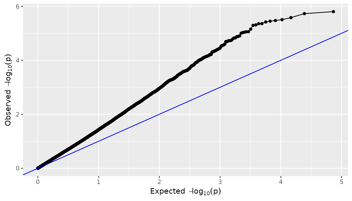

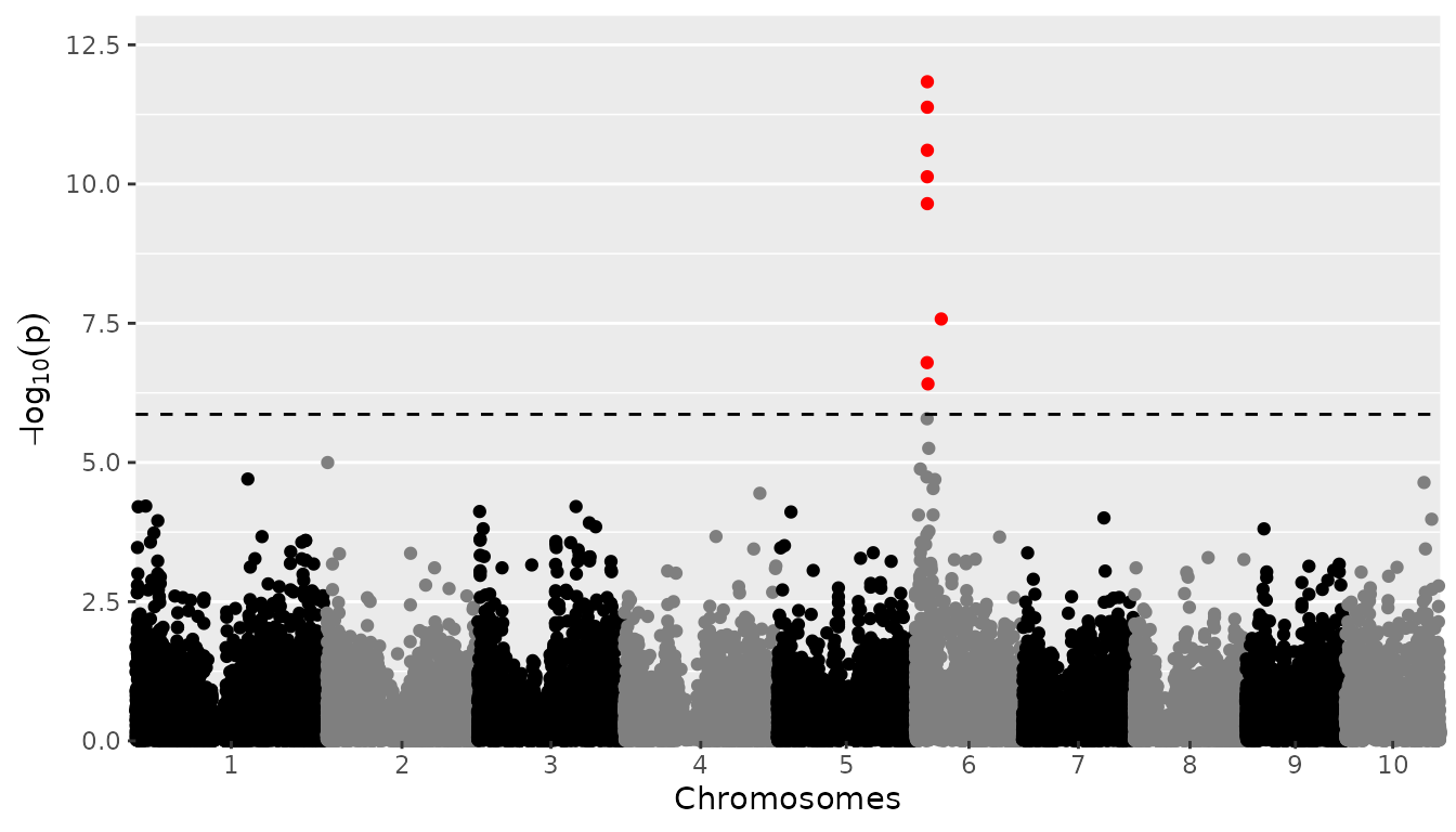
Manhattan plots

A Manhattan plot is made by setting plotType = "manhattan". Significant SNPs are marked in red.

## Plot a manhattan plot of GWAS Drops.
plot(GWASDrops, plotType = "manhattan")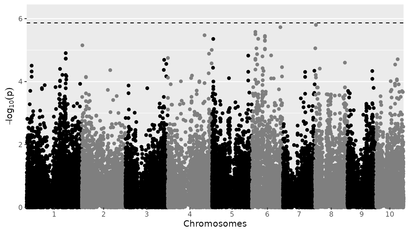

More options linked with plotType = "manhattan" are described in the statgenGWAS vignette.

QTL plots

A qtl plot can be made by setting plotType = "qtl". In this plot the significant SNPs are marked by circles at their genomic positions, with diameter proportional to the estimated effect size; for an example see Millet et al. (2016). Typically, this is done for multiple traits or environments, with the genomic position on the x-axis, which are displayed horizontally above each other and can thus be compared.

Since the traits are measured on a different scale, the effect estimates cannot be compared directly. For better comparison, one can set normalize = TRUE, which divides the estimates by the standard deviation of the phenotype.

## Plot a qtl plot of GWAS Drops for Mur13W.
## Set significance threshold to 5 and normalize effect estimates.
plot(GWASDrops, plotType = "qtl", yThr = 5, normalize = TRUE)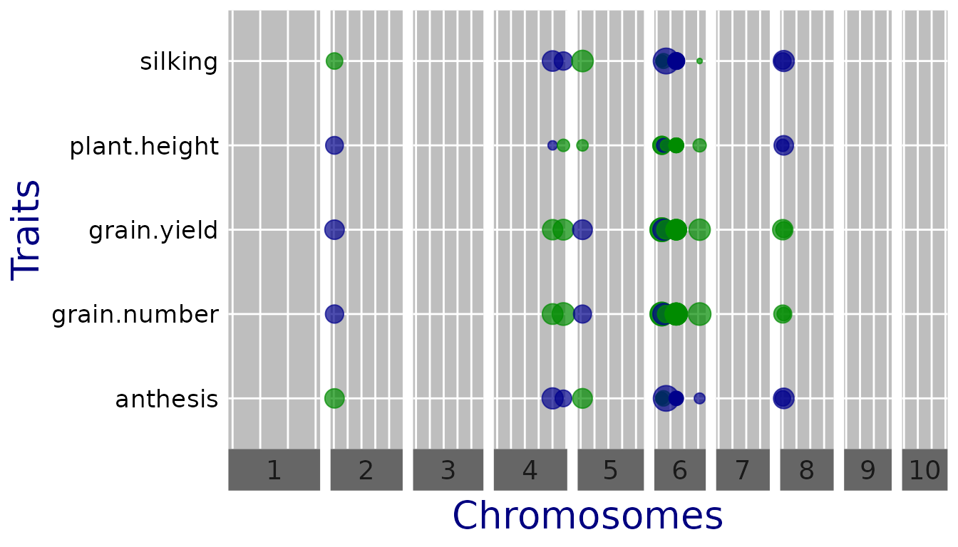

Other arguments can be used to plot a subset of the chromosomes (chr) and directly export the plot to .pptx (exportPptx = TRUE and specify pptxName). Note that the officer package is required for this. A full list of arguments can be found by running help(plot.GWAS).

Kinship matrices

The runMultiTraitGwas() function has an argument kinshipMethod, which defines the kinship matrix used for association mapping. Kinship matrices can be computed directly using the kinship function or within the runMultiTraitGwas function. There are five options: (1) using the covariance between the scaled SNP-scores (kinshipMethod = "astle", the default; see e.g. equation (2.2) in Astle and Balding (2009)) (2) Identity by State (kinshipMethod = "IBS"; see e.g. equation (2.3) in Astle and Balding (2009)) (3) using the formula by VanRaden (2008) (kinshipMethod = "vanRaden") (4) using an identity matrix (kinshipMethod = "identity"), corresponding to no kinship correction (5) User-defined, in which case the argument kin needs to be specified.

By default, the same kinship matrix is used for testing all SNPs (GLSMethod = "single"). When GLSMethod = "multi", the kinship matrix is chromosome-specific. In this case, the function fits variance components and computes effect-estimates and P-values for each chromosome in turn, using the kinship matrix for that chromosome (i.e. using all SNPs that are not on this chromosome). Each chromosome-specific kinship matrix is computed using the method specified by the argument kinshipMethod. As shown by Rincent et al. (2014), this can give a considerable improvement in power.

## Run multi-trait GWAS for trial 'Mur13W'.
## Use chromosome specific kinship matrices computed using method of van Raden.
GWASDropsChrSpec <- runMultiTraitGwas(gData = gDataDropsDedup, 
                                      trials = "Mur13W",
                                      GLSMethod = "multi",
                                      kinshipMethod = "vanRaden",
                                      covModel = "fa")

Worked example 2: one trait measured in multiple trials

Create gData object

In this example, we will focus on one trait, grain yield, in all trials. dropsPheno contains genotypic means for 10 trials. To be able to run a GWAS analysis with one trait measured in all trials, the data has to be reshaped and added as a single data.frame with “genotype” as first column and traits after that.

## Reshape phenotypic data to data.frame in wide format containing only grain.yield.
phenoDat <- reshape(dropsPheno[, c("Experiment", "genotype", "grain.yield")], 
                    timevar = "Experiment", 
                    idvar = "genotype", 
                    direction = "wide", 
                    v.names = "grain.yield")
## Rename columns to trial name only.
colnames(phenoDat)[2:ncol(phenoDat)] <-
  gsub(pattern = "grain.yield.", replacement = "",
       x = colnames(phenoDat)[2:ncol(phenoDat)])

Now we create a gData object containing map marker information and phenotypes.

## Create a gData object containing map, marker and phenotypic information.
gDataDropsxE <- statgenGWAS::createGData(geno = dropsMarkers,
                                         map = dropsMap, 
                                         pheno = phenoDat)
summary(gDataDropsxE)
#> map
#>  Number of markers: 41722 
#>  Number of chromosomes: 10 
#> 
#> markers
#>  Number of markers: 41722 
#>  Number of genotypes: 246 
#>  Content:
#>   0 1 2 NA 
#>   0.28 0.01 0.71 0 
#> 
#> pheno
#>  Number of trials: 1 
#> 
#>  phenoDat:
#>      Number of traits: 10 
#>      Number of genotypes: 246 
#> 
#>         Kar12W Gai12W Kar13W Ner12R Mar13R Mur13R Cra12R Cam12R Kar13R Mur13W
#> Min.       5.4    7.5    4.1    2.1    3.8    2.1  0.088   0.38    5.6    3.3
#> 1st Qu.    8.8   10.4    7.0    4.0    7.0    5.8  0.891   1.33    8.7    6.3
#> Median     9.9   11.2    7.9    4.7    7.7    6.9  1.381   1.87    9.8    7.5
#> Mean       9.7   11.2    8.0    4.7    7.8    6.9  1.492   1.98    9.9    7.4
#> 3rd Qu.   10.7   12.0    9.1    5.3    8.6    7.8  1.971   2.59   11.0    8.4
#> Max.      13.1   14.3   12.7    7.1   11.5   10.6  4.979   4.90   13.8   11.4
#> NA's       0.0    0.0    0.0    0.0    0.0    0.0  0.000   0.00    0.0    0.0

Recoding and cleaning of markers

## Remove duplicate SNPs from gDataDrops.
gDataDropsDedupxE <- statgenGWAS::codeMarkers(gDataDropsxE, 
                                              impute = FALSE,
                                              verbose = TRUE) 
#> Input contains 41722 SNPs for 246 genotypes.
#> 0 genotypes removed because proportion of missing values larger than or equal to 1.
#> 0 SNPs removed because proportion of missing values larger than or equal to 1.
#> 5098 duplicate SNPs removed.
#> Output contains 36624 SNPs for 246 genotypes.

Multi-trial GWAS

Similar to the first example we run a multi-trial GWAs using a factor analytic model.

## Run multi-trial GWAS for one trait in all trials.
GWASDropsxE <- runMultiTraitGwas(gData = gDataDropsDedupxE, 
                                 covModel = "fa")

Among the significant SNPs we find the large QTL on chromosome 6 reported in Millet et al. (2016).

head(GWASDropsxE$signSnp$pheno, row.names = FALSE)
#>              snp  trait chr      pos  pValue  LOD effect effectSe allFreq       snpStatus propSnpVar
#> 1:      SYN25281 Kar12W   6 18646369 1.6e-07  6.8   0.23    0.100    0.79 significant SNP      0.017
#> 2: PZE-106021363 Kar12W   6 18846283 7.4e-11 10.1   0.28    0.091    0.70 significant SNP      0.034
#> 3: PZE-106021410 Kar12W   6 18990291 2.5e-11 10.6   0.30    0.091    0.70 significant SNP      0.037
#> 4: PZE-106021419 Kar12W   6 18991091 1.5e-12 11.8   0.26    0.092    0.74 significant SNP      0.026
#> 5: PZE-106021420 Kar12W   6 18991117 2.2e-10  9.6   0.27    0.091    0.70 significant SNP      0.032
#> 6: PZE-106021424 Kar12W   6 18991481 4.2e-12 11.4   0.24    0.092    0.74 significant SNP      0.022

GWAS Summary

For a quick overview of the results, e.g. the number of significant SNPs, we again use the summary function. We restrict the output to two trials using the traits argument.

summary(GWASDropsxE, traits = c("Mur13W", "Kar12W"))
#> phenoDat:
#>  Traits analysed: Cam12R, Cra12R, Gai12W, Kar12W, Kar13R, Kar13W, Mar13R, Mur13R, Mur13W, Ner12R 
#> 
#>  Data are available for 36624 SNPs.
#>   0 of them were not analyzed because their minor allele frequency is below 0.01 
#> 
#>  GLSMethod: single 
#> 
#>  Trait: Mur13W 
#> 
#>      LOD-threshold: 5.9 
#>      Number of significant SNPs: 8 
#>      Smallest p-value among the significant SNPs: 1.5e-12 
#>      Largest p-value among the significant SNPs: 3.9e-07 (LOD-score: 6.4)
#> 
#>      No genomic control correction was applied
#>      Genomic control inflation-factor: 0.94 
#> 
#>  Trait: Kar12W 
#> 
#>      LOD-threshold: 5.9 
#>      Number of significant SNPs: 8 
#>      Smallest p-value among the significant SNPs: 1.5e-12 
#>      Largest p-value among the significant SNPs: 3.9e-07 (LOD-score: 6.4)
#> 
#>      No genomic control correction was applied
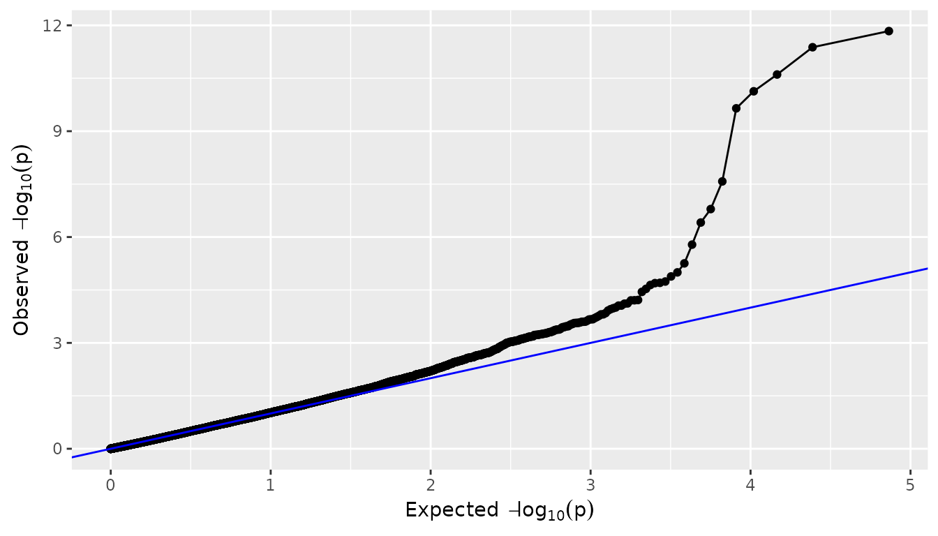
#>      Genomic control inflation-factor: 0.94

GWAS Plots

As in the first example we use the plot.GWAS() function to visualize the results in GWASDropsxE, with a QQ-plot, Manhattan plot or QTL-plot.

QQ plots

plot(GWASDropsxE, plotType = "qq")

Manhattan plots

plot(GWASDropsxE, plotType = "manhattan")

QTL plots

The trait is measured with the same scale across trials so the effect estimates can be compared directly (one can set normalize = FALSE).

## Set significance threshold to 6 and do not normalize effect estimates.
plot(GWASDropsxE, plotType = "qtl", yThr = 6, normalize = FALSE)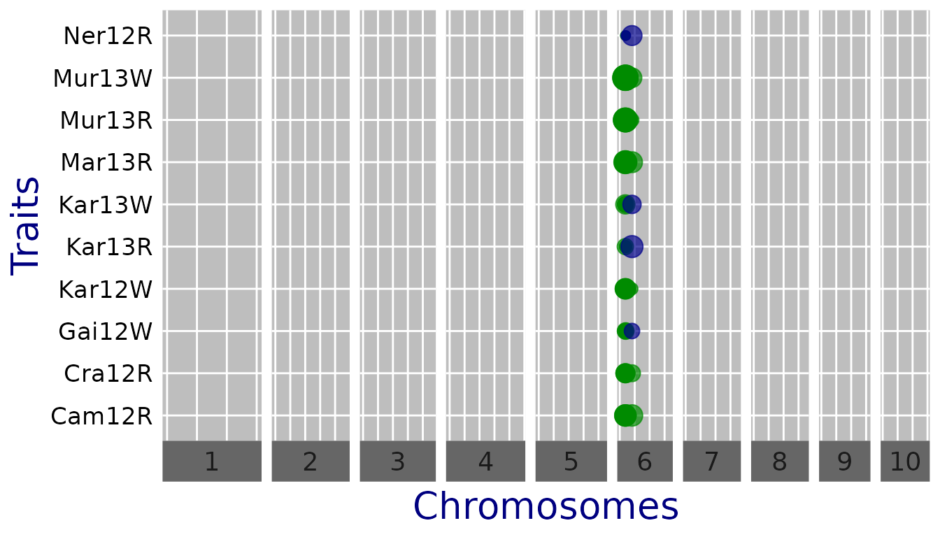

Further options

The runMultiTraitGwas() function has many more arguments that can be specified. In this section similar arguments are grouped and explained with examples on how to use them.

Significance thresholds

The threshold for selecting significant SNPs in a GWAS analysis is computed by default using Bonferroni correction, with an alpha of 0.05. The alpha can be modified setting the option alpha when calling runMultiTraitGwas(). Two other threshold types can be used: a fixed threshold (thrType = "fixed") specifying the $-\log_{10}(p)$ (LODThr) value of the threshold, or a threshold that defines the n SNPs with the highest $-\log_{10}(p)$ scores as significant SNPs. Set thrType = "small" together with nSnpLOD = n to do this. In the following example, we define all SNPs with $p < 10^{-4}$ as significant SNPs.

## Run multi-trait GWAS for Mur13W.
## Use a fixed significance threshold of 4.
GWASDropsFixThr <- runMultiTraitGwas(gData = gDataDropsDedup,
                                     trials = "Mur13W", 
                                     covModel = "fa",
                                     thrType = "fixed",
                                     LODThr = 4)

Controlling false discovery rate

A final option for selecting significant SNPs is by setting thrType = "fdr". When doing so the significant SNPs won’t be selected by computing a genome wide threshold, but by trying to control the rate of false discoveries as in Brzyski et al. (2016).

First, a list is defined containing all SNPs with a P-value below pThr, default 0.05. Then clusters of SNPs are created using a two step iterative process in which SNPs with the lowest P-values are selected as cluster representatives. This SNP and all SNPs that have a correlation with this SNP of $\rho$ or higher (specified by the function argument rho, default 0.4) will form a cluster. The selected SNPs are removed from the list and the procedure is repeated until no SNPs are left. At the end of this step, one has a list of clusters, with corresponding vector of P-values of the cluster representatives. Finally, to determine the number of significant clusters, the first cluster is determined for which the P-value of the cluster representative is larger than $cluster_{number} * \alpha / m$, where $m$ is the number of SNPs and $\alpha$ can be specified by the corresponding function argument. All previous clusters are selected as significant.

Variance components

There are three ways to compute the variance components used in the GWAS analysis. These can be specified by setting the argument covModel. See Models for the genetic and residual covariance for a description of the options.

Note that covModel = unst can only be used for less than 10 traits or trials. It is not recommended to use it for six to nine trials for computational reasons.

## Run multi-trait GWAS for for Mur13W.
## Use a factor analytic model for computing the variance components.
GWASDropsFA <- runMultiTraitGwas(gData = gDataDropsDedup,
                                 trials = "Mur13W",
                                 covModel = "fa")

## Rerun the analysis, using the variance components computed in the 
## previous model as inputs.
GWASDropsFA2 <- runMultiTraitGwas(gData = gDataDropsDedup,
                                  trials = "Mur13W",
                                  fitVarComp  = FALSE,
                                  Vg = GWASDropsFA$GWASInfo$varComp$Vg,
                                  Ve = GWASDropsFA$GWASInfo$varComp$Ve)

Parallel computing

To improve performance when using a pairwise variance component model, it is possible to use parallel computing. To do this, a parallel back-end has to be specified by the user, e.g. by using registerDoParallel from the doParallel package (see the example below). In addition, in the runMultiTraitGwas() function the argument parallel has to be set to TRUE. With these settings the computations are done in parallel per pair of traits.

## Register parallel back-end with 2 cores.
doParallel::registerDoParallel(cores = 2)

## Run multi-trait GWAS for one trait in all trials.
GWASDropsxEPar <- runMultiTraitGwas(gData = gDataDropsDedupxE,
                                    covModel = "pw",
                                    parallel = TRUE)

Covariates

Covariates can be included as extra fixed effects in the GWAS model. The runMultiTraitGwas() function distinguishes between ‘usual’ covariates and SNP-covariates. The former could be design factors such as block, or other traits one wants to condition on. In the latter case, the covariate(s) are one or more of the markers contained in the genotypic data. SNP-covariates can be set with the argument snpCov, which should be a vector of marker names. Similarly, other covariates should be specified using the argument covar, containing a vector of covariate names. The gData object should contain these covariates in gData$covar.

In case SNP-covariates are used, GWAS for all the other SNPs is performed with the the SNP-covariates as extra fixed effect; also the null model used to estimate the variance components includes these effects. For each SNP in SNP-covariates, a P-value is obtained using the same F-test and null model to estimate the variance components, but with only all other SNPs (if any) in SNP-covariates as fixed effects.

## Run multi-trait GWAS for Mur13W.
## Use PZE-106021410, the most significant SNP, as SNP covariate.
GWASDropsSnpCov <- runMultiTraitGwas(gData = gDataDropsDedup,
                                     trials = "Mur13W",
                                     snpCov = "PZE-106021410",
                                     covModel = "fa")

Minor Allele Frequency

It is recommended to remove SNPs with a low minor allele frequency (MAF) from the data before starting a GWAS analysis. However it is also possible to do so in the analysis itself. The difference between these approaches is that codeMarkers() removes the SNPs, whereas runMultiTraitGwas() excludes them from the analysis but leaves them in the output (with results set to NA). In the latter case it will still be possible to see the allele frequency of the SNP.
By default all SNPs with a MAF lower than 0.01 are excluded from the analysis. This can be controlled by the argument MAF. Setting MAF to 0 will still exclude duplicate SNPs since duplicates cause problems when fitting the underlying models.

## Run multi-trait GWAS for Mur13W.
## Only include SNPs that have a MAF of 0.05 or higher.
GWASDropsMAF <- runMultiTraitGwas(gData = gDataDropsDedup,
                                  trials = "Mur13W",
                                  covModel = "fa",
                                  MAF = 0.05)

Estimation of common SNP effects and QTL×E effects.

Besides a normal SNP-effect model, it is possible to fit a common SNP-effect model as well (see Hypotheses for the SNP-effects). When doing so, in addition to the SNP-effect, also the common SNP-effect and the QTL×E effect and corresponding standard errors and P-values are returned. These are included as extra columns in the GWAResult data.table in the output of the function.

## Run multi-trait GWAS for Mur13W.
## Fit an additional common sNP effect model.
GWASDropsCommon <- runMultiTraitGwas(gData = gDataDropsDedup,
                                     trials = "Mur13W",
                                     covModel = "fa",
                                     estCom = TRUE)
head(GWASDropsCommon$GWAResult$Mur13W)
#>              snp    trait chr    pos pValue    LOD effect effectSe allFreq pValCom effsCom effsComSe pValQtlE
#> 1:         SYN83 anthesis   1   3498   0.98 0.0087  -0.12     0.19    0.60   0.536  -0.028     0.045     0.98
#> 2: PZE-101000060 anthesis   1 157104   0.20 0.6991   0.47     0.20    0.72   0.029   0.103     0.048     0.58
#> 3: PZE-101000088 anthesis   1 238347   0.19 0.7142  -0.61     0.25    0.84   0.049  -0.115     0.059     0.44
#> 4: PZE-101000083 anthesis   1 239225   0.76 0.1207  -0.16     0.18    0.58   0.203  -0.054     0.043     0.88
#> 5: PZE-101000108 anthesis   1 255850   0.60 0.2253   0.15     0.34    0.90   0.774  -0.023     0.079     0.48
#> 6: PZE-101000111 anthesis   1 263938   0.60 0.2217  -0.37     0.24    0.83   0.248  -0.064     0.055     0.66

The SNPs with a significant QTLxE effect come from the same regions as the SNPs in supplementary table 6 in Millet et al. (2016), who however used a different SNP set. Another difference is that here we explicitly test for QTLxE within the GWAS, whereas Millet et al. (2016) regressed SNP effects on environmental covariates.

References

Astle, William, and David J. Balding. 2009. “Population Structure and Cryptic Relatedness in Genetic Association Studies.” Statistical Science 24 (4): 451–71. https://doi.org/10.1214/09-sts307.

Brzyski, Damian, Christine B. Peterson, Piotr Sobczyk, Emmanuel J. Candès, Malgorzata Bogdan, and Chiara Sabatti. 2016. “Controlling the Rate of GWAS False Discoveries.” Genetics 205 (1): 61–75. https://doi.org/10.1534/genetics.116.193987.

Furlotte, N. A., and E. Eskin. 2015. “Efficient Multiple-Trait Association and Estimation of Genetic Correlation Using the Matrix-Variate Linear Mixed Model.” Genetics 200 (1): 59–68. https://doi.org/10.1534/genetics.114.171447.

Korte, Arthur, Bjarni J Vilhjálmsson, Vincent Segura, Alexander Platt, Quan Long, and Magnus Nordborg. 2012. “A Mixed-Model Approach for Genome-Wide Association Studies of Correlated Traits in Structured Populations.” Nature Genetics 44 (9): 1066–71. https://doi.org/10.1038/ng.2376.

Millet, Emilie J., Cyril Pommier, Mélanie Buy, Axel Nagel, Willem Kruijer, Therese Welz-Bolduan, Jeremy Lopez, et al. 2019. “A Multi-Site Experiment in a Network of European Fields for Assessing the Maize Yield Response to Environmental Scenarios.” Portail Data Inra. https://doi.org/10.15454/IASSTN.

Millet, Emilie J., Claude Welcker, Willem Kruijer, Sandra Negro, Stephane Nicolas, Sebastien Praud, Nicolas Ranc, et al. 2016. “Genome-Wide Analysis of Yield in Europe: Allelic Effects as Functions of Drought and Heat Scenarios.” Plant Physiology, July, pp.00621.2016. https://doi.org/10.1104/pp.16.00621.

Rincent, Renaud, Laurence Moreau, Hervé Monod, Estelle Kuhn, Albrecht E. Melchinger, Rosa A. Malvar, Jesus Moreno-Gonzalez, et al. 2014. “Recovering Power in Association Mapping Panels with Variable Levels of Linkage Disequilibrium.” Genetics 197 (1): 375–87. https://doi.org/10.1534/genetics.113.159731.

VanRaden, P. M. 2008. “Efficient Methods to Compute Genomic Predictions.” Journal of Dairy Science 91 (11): 4414–23. https://doi.org/10.3168/jds.2007-0980.

Zhou, Xiang, and Matthew Stephens. 2014. “Efficient Multivariate Linear Mixed Model Algorithms for Genome-Wide Association Studies.” Nature Methods 11 (4): 407–9. https://doi.org/10.1038/nmeth.2848.

Bart-Jan van Rossum

2024-01-23

Multi-Trait GWAS

Theoretical background

Hypotheses for the SNP-effects

Models for the genetic and residual covariance

The class `gData`

Worked example 1: multiple traits in one trial

Create gData object

Recoding and cleaning of markers

Running Multi-trait GWAS

GWAS Summary

GWAS Plots

QQ plots

Manhattan plots

QTL plots

Kinship matrices

Worked example 2: one trait measured in multiple trials

Create gData object

Recoding and cleaning of markers

Multi-trial GWAS

GWAS Summary

GWAS Plots

QQ plots

Manhattan plots

QTL plots

Further options

Significance thresholds

Variance components

Covariates

Minor Allele Frequency

Estimation of common SNP effects and QTL×E effects.

References

Multi-trait GWAS with the statgenQTLxT package

Bart-Jan van Rossum

2024-01-23

Multi-Trait GWAS

Theoretical background

Hypotheses for the SNP-effects

Models for the genetic and residual covariance

The class gData

Worked example 1: multiple traits in one trial

Create gData object

Recoding and cleaning of markers

Running Multi-trait GWAS

GWAS Summary

GWAS Plots

QQ plots

Manhattan plots

QTL plots

Kinship matrices

Worked example 2: one trait measured in multiple trials

Create gData object

Recoding and cleaning of markers

Multi-trial GWAS

GWAS Summary

GWAS Plots

QQ plots

Manhattan plots

QTL plots

Further options

Significance thresholds

Variance components

Covariates

Minor Allele Frequency

Estimation of common SNP effects and QTL×E effects.

References

The class `gData`