AMMI analysis

The Additive Main Effects and Multiplicative Interaction (AMMI) model fits a model which involves the Additive Main effects (i.e. genotype and trial) along with Multiplicative Interaction effects. The additive effects are the classical ANOVA main effects for genotype and environment, the multiplicative effects follow from a principal component analysis on the interaction residuals (= genotype by environment means after adjustment for additive genotype and environment effects). This results in an interaction characterized by Interaction Principal Components (IPCA) enabling simultaneous plotting of genotypes and trials.

The parameter nPC is used to indicate the number of principal components that is used in the principal component analysis (PCA). By setting this parameter to NULL the algorithm determines the best number of principal components (see Details).

By specifying the parameter byYear = TRUE, a separate analysis will be done for every year in the data. Combining the option with nPC = NULL may result in different numbers of principal components per year. The AMMI estimates will still be returned as a single data.frame, but the other results will be either lists or arrays.

Usage

gxeAmmi(
  TD,
  trials = names(TD),
  trait,
  nPC = 2,
  byYear = FALSE,
  center = TRUE,
  excludeGeno = NULL,
  useWt = FALSE
)

Arguments

TD: An object of class TD.
trials: A character string specifying the trials to be analyzed. If not supplied, all trials are used in the analysis.
trait: A character string specifying the trait to be analyzed.
nPC: An integer specifying the number of principal components used as multiplicative term of genotype-by-trial interaction. If NULL, the number of principal components is determined by the algorithm using forward selection. See details.
byYear: Should the analysis be done by year? If TRUE the data is split by the variable year, analysis is performed and the results are merged together and returned.
center: Should the variables be shifted to be zero centered?
excludeGeno: An optional character vector with names of genotypes to be excluded from the analysis. If NULL, all genotypes are used.
useWt: Should weighting be used when modeling? Requires a column wt in TD.

Value

An object of class AMMI, a list containing:

envScores: A matrix with environmental scores.
genoScores: A matrix with genotypic scores.
importance: A data.frame containing the importance of the principal components.
anova: A data.frame containing anova scores of the AMMI analysis.
fitted: A data.frame containing fitted values from the AMMI model.
trait: A character string containing the analyzed trait.
envMean: A numerical vector containing the environmental means.
genoMean: A numerical vector containing the genotypic means.
overallMean: A numerical value containing the overall mean.

If byYear = TRUE, all returned items in the AMMI object except fitted will consist of a list of results by year.

Details

First a linear model \(trait = genotype + trial + \epsilon\) is fitted with both genotype and trial fixed components in the model.
The residuals from the fitted model are then used in a PCA. If nPC is not NULL a single PCA is done using prcomp with maximum rank nPC.
In case nPC = NULL, the PCA is first done with one PC. Then using forward selection one by one the number of PCs is increased as long as the added component is significant in the analysis.
AMMI estimates are then computed using the results of the PCA.

References

Gauch H.G. (1992) Statistical Analysis of Regional Yield Trials: AMMI Analysis of Factorial Designs. Elsevier, Amsterdam.

Yan, W., Kang, M. (2002). GGE Biplot Analysis. Boca Raton: CRC Press.

Examples

## Run AMMI analysis on TDMaize.
geAmmi <- gxeAmmi(TD = TDMaize, trait = "yld")

## Summarize results.
summary(geAmmi)
#> Principal components 
#> ====================
#>                              PC1       PC2
#> Standard deviation     161.12397 136.06980
#> Proportion of Variance   0.29796   0.21250
#> Cumulative Proportion    0.29796   0.51046
#> 
#> Anova 
#> =====
#> Analysis of Variance Table
#> 
#> Response: yld
#>                Df    Sum Sq  Mean Sq   F value    Pr(>F)    
#> Trial           7 127771687 18253098 1466.4731 < 2.2e-16 ***
#> Genotype      210  13821018    65814    5.2876 < 2.2e-16 ***
#> Interactions 1470  18296997    12447                        
#> PC1           216   5451796    25240    2.9306 < 2.2e-16 ***
#> PC2           214   3888148    18169    2.1096  1.31e-14 ***
#> Residuals    1040   8957053     8613                        
#> ---
#> Signif. codes:  0 ‘***’ 0.001 ‘**’ 0.01 ‘*’ 0.05 ‘.’ 0.1 ‘ ’ 1
#> 
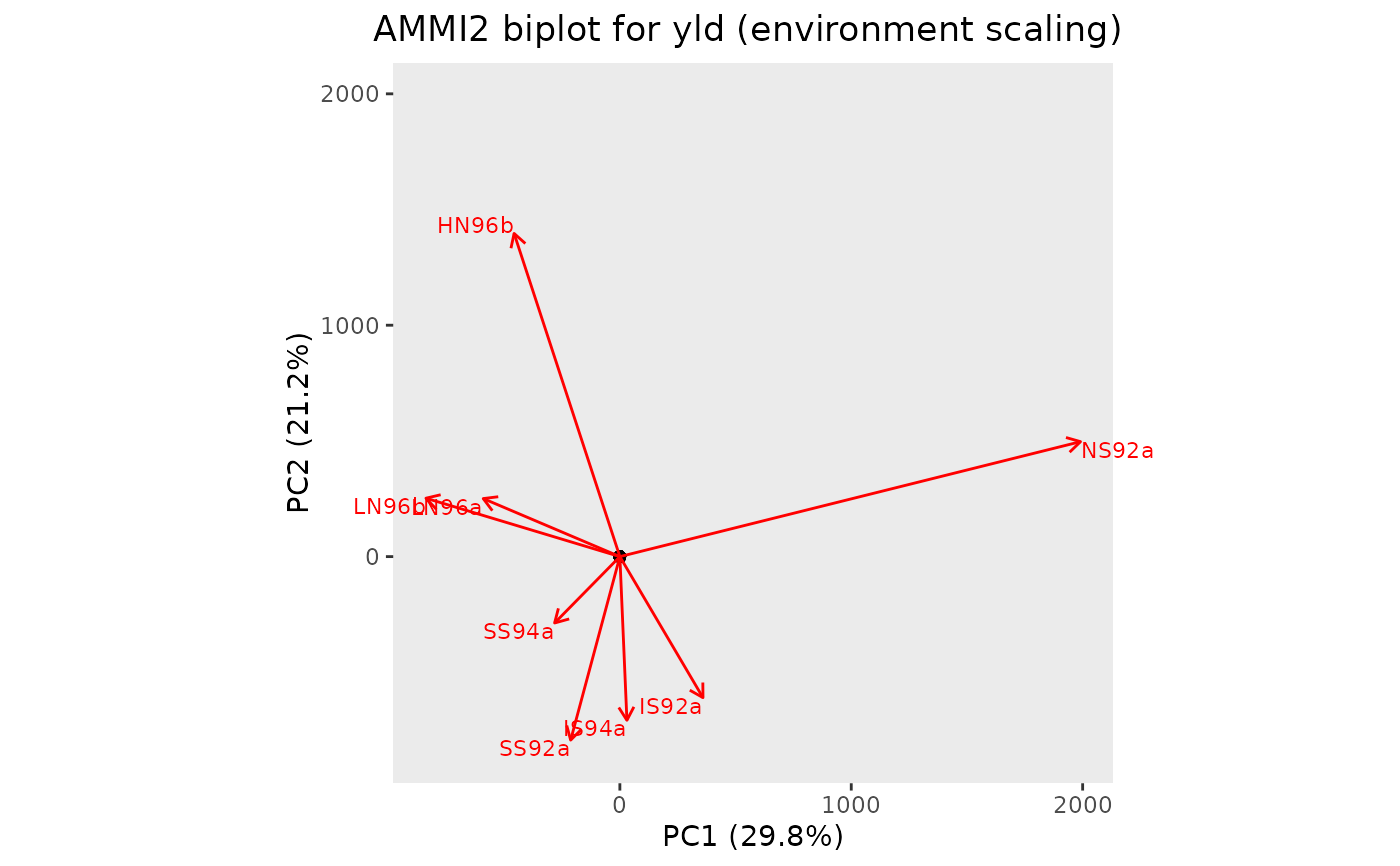
#> Environment scores 
#> ==================
#>               PC1        PC2
#> HN96b -0.19530892  0.7066260
#> IS92a  0.15345251 -0.3083436
#> IS94a  0.01300981 -0.3578091
#> LN96a -0.25229650  0.1268734
#> LN96b -0.35806958  0.1276750
#> NS92a  0.85058379  0.2513096
#> SS92a -0.09087845 -0.4011956
#> SS94a -0.12049264 -0.1451358

## Create a biplot of genotypes and environment interaction with PC1 and PC2.
plot(geAmmi, plotType = "AMMI2")


## Create a pdf report summarizing the results.
# \donttest{
report(geAmmi, outfile = tempfile(fileext = ".pdf"))
#> Error in report.AMMI(geAmmi, outfile = tempfile(fileext = ".pdf")): An installation of LaTeX is required to create a pdf report.
# }