Finlay-Wilkinson analysis

This function performs a Finlay-Wilkinson analysis of data classified by two factors.

Usage

gxeFw(
  TD,
  trials = names(TD),
  trait,
  maxIter = 15,
  tol = 0.001,
  sorted = c("descending", "ascending", "none"),
  genotypes = NULL,
  useWt = FALSE
)

Arguments

TD: An object of class TD.
trials: A character string specifying the trials to be analyzed. If not supplied, all trials are used in the analysis.
trait: A character string specifying the trait to be analyzed.
maxIter: An integer specifying the maximum number of iterations in the algorithm.
tol: A positive numerical value specifying convergence tolerance of the algorithm.
sorted: A character string specifying the sorting order of the estimated values in the output.
genotypes: An optional character string containing the genotypes to which the analysis should be restricted. If NULL, all genotypes are used.
useWt: Should weighting be used when modeling? Requires a column wt in TD.

Value

An object of class FW, a list containing:

estimates

A data.frame containing the estimated values, with the following columns:

genotype: The name of the genotype.
sens: The estimate of the sensitivity.
se_sens: The standard error of the estimate of the sensitivity.
genMean: The estimate of the genotypic mean.
se_genMean: The standard error of the estimate of the genotypic mean.
MSdeviation: The mean square deviation about the line fitted to each genotype
rank: The rank of the genotype based on its sensitivity.

anova

A data.frame containing anova scores of the FW analysis.

envEffs

A data.frame containing the environmental effects, with the following columns:

trial: The name of the trial.
envEff: The estimate of the environment effect.
se_envEff: The standard error of the estimate of the environment effect.
envMean: The estimate of the environment mean.
rank: The rank of the trial based on its mean.

TD

The object of class TD on which the analysis was performed.

fittedGeno

A numerical vector containing the fitted values for the genotypes.

trait

A character string containing the analyzed trait.

nGeno

A numerical value containing the number of genotypes in the analysis.

nEnv

A numerical value containing the number of environments in the analysis.

tol

A numerical value containing the tolerance used during the analysis.

iter

A numerical value containing the number of iterations for the analysis to converge.

References

Finlay, K.W. & Wilkinson, G.N. (1963). The analysis of adaptation in a plant-breeding programme. Australian Journal of Agricultural Research, 14, 742-754.

Examples

## Run Finlay-Wilkinson analysis on TDMaize.
geFW <- gxeFw(TDMaize, trait = "yld")
#> Warning: ANOVA F-tests on an essentially perfect fit are unreliable

## Summarize results.
summary(geFW)
#> Environmental effects 
#> =====================
#>   Trial     EnvEff SE_EnvEff   EnvMean SE_EnvMean Rank
#> 1 HN96b   25.61186  5.963951  481.7914   36.14588    3
#> 2 IS92a  182.26254  5.963951  638.4351   43.17104    2
#> 3 IS94a  -35.03765  5.963951  421.1446   36.28094    4
#> 4 LN96a -271.00666  5.963951  185.1862   50.51782    7
#> 5 LN96b -364.59899  5.963951   91.5981   59.74929    8
#> 6 NS92a  595.22993  5.963951 1051.3839   85.77817    1
#> 7 SS92a  -88.89999  5.963951  367.2847   37.82243    6
#> 8 SS94a  -43.56105  5.963951  412.6216   36.43858    5
#> 
#> Anova 
#> =====
#>                 Df    Sum Sq  Mean Sq   F value    Pr(>F)    
#> Trial            7 127771687 18253098 1753.1259 < 2.2e-16 ***
#> Genotype       210  13821018    65814    6.3212 < 2.2e-16 ***
#> Sensitivities  210   5178199    24658    2.3683 < 2.2e-16 ***
#> Residual      1260  13118797    10412                        
#> Total         1687 159889702    94778                        
#> ---
#> Signif. codes:  0 ‘***’ 0.001 ‘**’ 0.01 ‘*’ 0.05 ‘.’ 0.1 ‘ ’ 1
#> 
#> Most sensitive genotypes
#> ========================
#>  Genotype  GenMean SE_GenMean Rank     Sens   SE_Sens MSdeviation
#>      G091 510.4500   35.99027    1 1.440452 0.1308111    6109.574
#>      G194 521.4250   35.99027    2 1.427522 0.1308111    4836.093
#>      G055 616.8500   35.99027    3 1.418572 0.1308111    7160.220
#>      G042 561.3875   35.99027    4 1.397123 0.1308111   18919.353
#>      G103 510.8000   35.99027    5 1.389754 0.1308111    9408.329

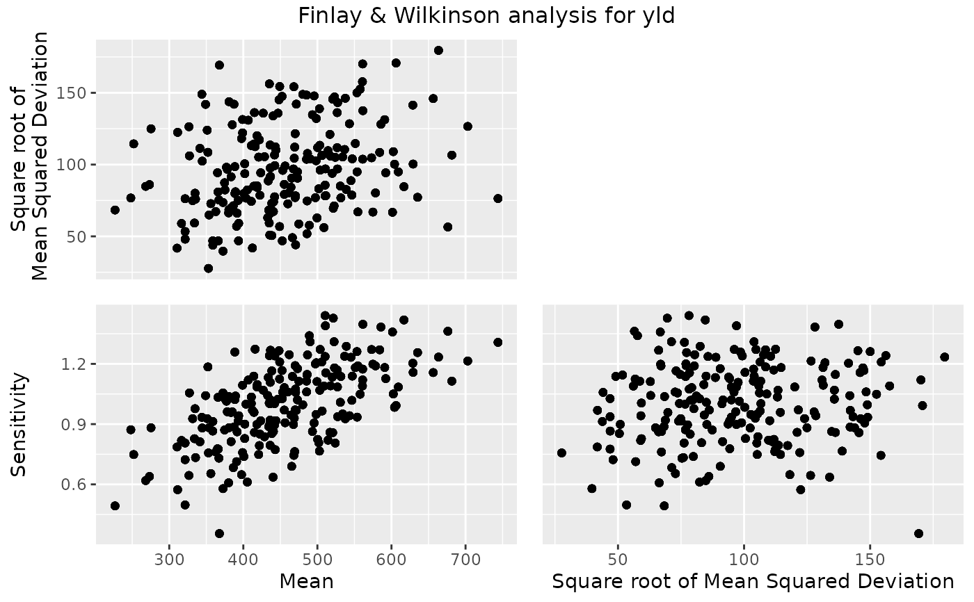
## Create a scatterplot of the results.
plot(geFW, plotType = "scatter")


# \donttest{
## Create a report summarizing the results.
report(geFW, outfile = tempfile(fileext = ".pdf"))
#> Error in report.FW(geFW, outfile = tempfile(fileext = ".pdf")): An installation of LaTeX is required to create a pdf report.
# }

Usage

Arguments

Value

References

See also

Examples