Fit Splines

Fit P-Splines on corrected or raw data. The number of knots is chosen by the user. The function outputs are predicted P-Spline values and their first and second derivatives on a dense grid. The outputs can then be used for outlier detection for time series (see detectSerieOut) and to estimate relevant parameters from the curve for further analysis (see estimateSplineParameters).

Usage

fitSpline(
  inDat,
  trait,
  genotypes = NULL,
  plotIds = NULL,
  knots = 50,
  useTimeNumber = FALSE,
  timeNumber = NULL,
  minNoTP = NULL
)

Arguments

inDat: A data.frame with corrected spatial data.
trait: A character string indicating the trait for which the spline should be fitted.
genotypes: A character vector indicating the genotypes for which splines should be fitted. If NULL, splines will be fitted for all genotypes.
plotIds: A character vector indicating the plotIds for which splines should be fitted. If NULL, splines will be fitted for all plotIds.
knots: The number of knots to use when fitting the spline.
useTimeNumber: Should the timeNumber be used instead of the timePoint?
timeNumber: If useTimeNumber = TRUE, a character vector indicating the column containing the numerical time to use.
minNoTP: The minimum number of time points for which data should be available for a plant. Defaults to 80% of all time points present in the TP object. No splines are fitted for plants with less than the minimum number of timepoints.

Value

An object of class HTPSpline, a list with two data.frames, predDat with predicted values and coefDat

with P-Spline coefficients on a dense grid.

Examples

## The data from the Phenovator platform have been corrected for spatial
## trends and outliers for single observations have been removed.

## Fit P-Splines on a subset of genotypes
subGeno <- c("G070", "G160")
fit.spline <- fitSpline(inDat = spatCorrectedVator,
                        trait = "EffpsII_corr",
                        genotypes = subGeno,
                        knots = 50)

## Extract the data.frames with predicted values and P-Spline coefficients.
predDat <- fit.spline$predDat
head(predDat)
#>   timeNumber           timePoint pred.value         deriv       deriv2 plotId
#> 1          0 2018-05-31 16:37:00  0.6687993 -8.426473e-07 1.839623e-12 c10r29
#> 2        800 2018-05-31 16:50:20  0.6681258 -8.410810e-07 2.076021e-12 c10r29
#> 3       1600 2018-05-31 17:03:40  0.6674536 -8.393257e-07 2.312419e-12 c10r29
#> 4       2400 2018-05-31 17:17:00  0.6667829 -8.373812e-07 2.548817e-12 c10r29
#> 5       3200 2018-05-31 17:30:20  0.6661139 -8.352475e-07 2.785215e-12 c10r29
#> 6       4000 2018-05-31 17:43:40  0.6654466 -8.329248e-07 3.021613e-12 c10r29
#>   genotype
#> 1     G160
#> 2     G160
#> 3     G160
#> 4     G160
#> 5     G160
#> 6     G160

coefDat <- fit.spline$coefDat
head(coefDat)
#>   obj.coefficients plotId        type genotype
#> 1        0.6965965 c10r29 timeNumber1     G160
#> 2        0.6685027 c10r29 timeNumber2     G160
#> 3        0.6421887 c10r29 timeNumber3     G160
#> 4        0.6265465 c10r29 timeNumber4     G160
#> 5        0.6263577 c10r29 timeNumber5     G160
#> 6        0.6420706 c10r29 timeNumber6     G160

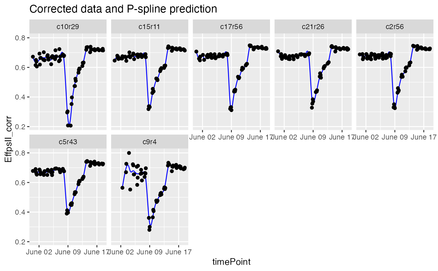
## Visualize the P-Spline predictions for one genotype.
plot(fit.spline, genotypes = "G160")


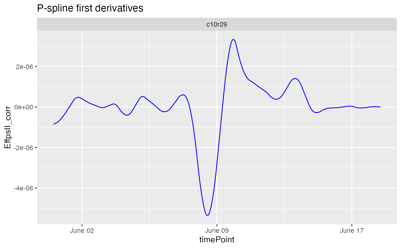
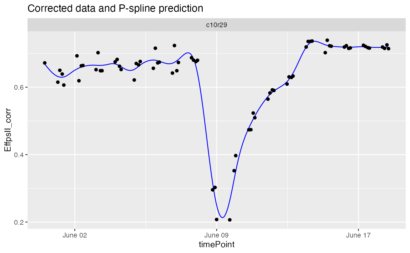
## Visualize the P-Spline predictions and first derivatives for one plant.
plot(fit.spline, plotIds = "c10r29", plotType = "predictions")

plot(fit.spline, plotIds = "c10r29", plotType = "derivatives")

Usage

Arguments

Value

See also

Examples