Modeling field trials using statgenSTA

The statgenSTA Package

The statgenSTA (Single Trial Analysis) package is developed as an easy-to-use package for analyzing data of plant breeding experiments with many options for plotting and reporting the results of the analyses. The package can be used for visualizing trial data, analyzing data per trial and automatically creating reports of the analysis.

This vignette describes in detail how to prepare data for analysis, perform analyses using different modeling engines, and extract the results from the models.

Data preparation

The first step, when modeling field trial data with the statgenSTA package, is creating an object of class TD (Trial Data). This object is used throughout the statgenSTA package as input for analyses. From here onwards, an object of class TD will be referred to as a TD object.

Creating a `TD` object

A TD object can be created from a data.frame with the function createTD(). This function does a number of things:

Rename columns to default column names used by the functions in the statgenSTA package. For example, the column in the data containing variety/accession/genotype is renamed to “genotype”. Original column names are stored as an attribute of the TD object.
Convert column types to the default column types. For example, the column “genotype” is converted to a factor and “rowCoord” to a numeric column.
Split the data into separate data.frames by trial. A TD object is a list of data.frames where each data.frame contains the data for a single trial. If there is only one trial or no column trial is defined, the output will be a list with only one item.
Add metadata to the TD object. This metadata is used to store background information about the trials. It consists of location, date of the experiment, longitude, latitude, trial design, plot width, and plot length. None of these are strictly necessary for any analysis and metadata can, therefore, be safely ignored. However, the metadata is used when plotting field layouts, plotting trials on a map, and naming plots. Metadata can be added when creating the TD object using the appropriate arguments in createTD() (see Example). It is also possible to first create a TD object without metadata and then add metadata using the getMeta() and setMeta() functions (see Metadata). After creating a TD object, data for new trials can be added to it using addTD(). This function works similarly as createTD() except that it adds data to an existing TD object instead of creating a new one.
Dropping one or more trials from a TD object can be achieved by using the function dropTD().

When using check genotypes, the genotype and checkId have to be specified in a specific way to assure the models are fitted correctly. The column genotype should contain NA for the check genotypes. The column checkId should contain one value for the regular genotypes, e.g. noCheck, and the name of the genotype for the checks. An example of this layout is in the table below.

genotype	checkId
G₁	noCheck
G₂	noCheck
…	noCheck
G_n-1	noCheck
G_n	noCheck
NA	check₁
NA	check₂
…	…
NA	check_m-1
NA	check_m

Note that fitting models with check genotypes can only be done in this way when genotype is fitted as random effect. When fitting models with genotype as fixed effect both regular and check genotypes should be specified in the genotype column.

Example

The use of the package is demonstrated using maize data from the European Union project DROPS (https://cordis.europa.eu/project/id/244374). The data is available from https://doi.org/10.15454/IASSTN (E. J. Millet et al. 2019) and the relevant data set is included as data.frame in the statgenSTA package.

The first step is loading the data into R.

data(dropsRaw)

The object named dropsRaw contains data for 256 maize hybrids, grown with two water regimes (irrigated or rainfed), in seven fields in 2012 and 2013. The hybrids are divided in four families. A selection of ten experiments and eight traits is made from the full data set. These ten experiments form a good representation of the full set of experiments covering the five scenarios described in E. Millet et al. (2016). Throughout this vignette in all examples the trait grain.yield will be analyzed. For a more detailed description of the contents of the data see help(dropsRaw).

For the example, first a TD object is created for experiments conducted in 2012. The data for 2013 is then added later on. In practice all this could be done in one go.

## Create a TD object containing data for 2012.
dropsTD <- createTD(data = dropsRaw[dropsRaw$year == 2012, ],
                    genotype = "Variety_ID", 
                    trial = "Experiment",
                    loc = "Site",
                    repId = "Replicate", 
                    subBlock = "block",
                    rowCoord = "Row", 
                    colCoord = "Column", 
                    trLat = "Lat", 
                    trLong = "Long")

The TD object just created is a list with five items, one for each trial (combination of location, year and water regime) in the original data.frame. The column “Variety_ID” in the original data is renamed to “genotype” and converted to a factor. The columns “Replicate”, “block”, “loc” are renamed and converted likewise. The columns “Row” and “Column” are renamed to “rowCoord” and “colCoord” respectively. Simultaneously two columns “rowId” and “colId” are created containing the same information converted to a factor. This seemingly duplicate information is needed for spatial analysis. It is possible to define different columns as “rowId” and “colId” than the ones used as “rowCoord” and “colCoord”. Finally, the latitude and longitude of the trials is read from the column “Lat” and “Long” in the input and stored in a TD object named dropsTD. The information about which columns have been renamed, when creating a TD object, is stored as an attribute of each individual data.frame in the object.

Metadata

The metadata will be a data.frame with five rows, one for each trial in the object named dropsTD. The data.frame has the following columns:

	Content	Usage
trLocation	Location	Default names for plots and reports
trDate	Date
trDesign	Design	Model specification (see Model types)
trLat	Latitude	Position in a map plot (see Map plot)
trLong	Longitude	Position in a map plot (see Map plot)
trPlWidth	Plot width	Ratio of width/height in a layout plot (see Layout plot)
trPlLength	Plot length	Ratio of width/height in a layout plot (see Layout plot)

## Extract metadata from the TD object. 
(dropsMeta <- getMeta(TD = dropsTD))
#>        trLocation trDate trDesign  trLat trLong trPlWidth trPlLength
#> Cam12R Campagnola   <NA>       NA 45.171  9.532        NA         NA
#> Cra12R    Craiova   <NA>       NA 44.116 24.348        NA         NA
#> Gai12W    Gaillac   <NA>       NA 43.910  1.890        NA         NA
#> Kar12W  Karlsruhe   <NA>       NA 49.100  8.320        NA         NA
#> Ner12R      Nerac   <NA>       NA 44.170  0.307        NA         NA

After extracting the metadata, it can be modified and then added back to the original TD object.

## Set trial data as 1-1-2012.
dropsMeta$trDate <- as.Date(rep("010112", times = 5), "%d%m%y")
dropsTD <- setMeta(TD = dropsTD, meta = dropsMeta)

Add extra data to a `TD` object

To add the data for the 2013 trials to the TD object the function addTD() can be used. This function is very similar to createTD(). The only exception is, that a TD object has to be specified to which the new data is added.

## Add the data for the 2013 trials to the TD object.
dropsTD <- addTD(TD = dropsTD, 
                 data = dropsRaw[dropsRaw$year == 2013, ],
                 genotype = "Variety_ID", 
                 trial = "Experiment",
                 loc = "Site", 
                 repId = "Replicate", 
                 subBlock = "block",
                 rowCoord = "Row", 
                 colCoord = "Column", 
                 trLat = "Lat", 
                 trLong = "Long")

## Inspect the metadata after the extra trial was added.
getMeta(TD = dropsTD)
#>         trLocation     trDate trDesign  trLat trLong trPlWidth trPlLength
#> Cam12R  Campagnola 2012-01-01       NA 45.171  9.532        NA         NA
#> Cra12R     Craiova 2012-01-01       NA 44.116 24.348        NA         NA
#> Gai12W     Gaillac 2012-01-01       NA 43.910  1.890        NA         NA
#> Kar12W   Karlsruhe 2012-01-01       NA 49.100  8.320        NA         NA
#> Ner12R       Nerac 2012-01-01       NA 44.170  0.307        NA         NA
#> Kar13R   Karlsruhe       <NA>       NA 49.100  8.320        NA         NA
#> Kar13W   Karlsruhe       <NA>       NA 49.100  8.320        NA         NA
#> Mar13R Martonvasar       <NA>       NA 47.311 18.778        NA         NA
#> Mur13R      Murony       <NA>       NA 46.780 21.050        NA         NA
#> Mur13W      Murony       <NA>       NA 46.780 21.050        NA         NA

Note that the metadata now contains information about all ten trials. Only for the 2012 trials the trial date is filled. Since this information is not used in any of the analyses in the package we leave this.

Summarizing a `TD` object

The summary() function can be used to get an idea of the content of the data in the TD object. Multiple traits can be summarized at once, but for clarity here a summary is only made for grain.yield of a single trial.

## Create a summary for grain yield in Gai12W.
summary(dropsTD, 
        trial = "Gai12W", 
        traits = "grain.yield")
#> 
#> Summary statistics for grain.yield in Gai12W  
#> 
#>                          grain.yield
#> Number of observations         483.0
#> Number of missing values        19.0
#> Mean                           11.23
#> Median                         11.22
#> Min                             6.71
#> Max                            14.68
#> First quantile                 10.38
#> Third quantile                 12.09
#> Variance                       1.845

Using the default argument settings nine summary statistics are printed, but many more are available. These can be accessed using the argument what in the summary() function. For a full list of available statistics, use help(summary.TD). It is also possible to output all statistics using what = "all".

It is possible to summarize the data in a TD object for different groups. This can be done by using the argument groupBy. It will display three main summary statistics per group. Again, more statistics can be displayed using the argument what.

## Create a summary per family in Gai12W
summary(dropsTD, 
        trial = "Gai12W", 
        traits = "grain.yield", 
        groupBy = "geneticGroup")
#> 
#> Summary statistics for grain.yield in Gai12W grouped by geneticGroup 
#> 
#>                        Stiff_Stalk Iodent Other Lancaster
#> Number of observations       107.0   79.0 210.0      87.0
#> Mean                         11.85  11.42 10.61     11.80
#> Standard deviation           1.320  0.964 1.337     1.110

Plotting a `TD` object

Several plots can be made to further investigate the contents of a TD object.

a layout plot showing the layout of the trial
a map plot showing the location of the trials on a geographical map
a box plot showing the variability of the traits
a correlation plot showing the correlation of values for a trait between trials
a scatter plot showing the scatter plot for a trait between pairs of trials

All plots are described in detail in the sections below.

In all plots the default colors for both genotype groups and trial groups are chosen from a predefined color palette. For genotype groups the color palette is “Dark 2”, for trial groups it is “Alphabet”. See here for an overview of these colors.

It is possible to specify different colors for genotype groups and trial groups per plot using the arguments colGeno and colTrial respectively. Also, more conveniently, the default colors can be set using the options statgen.genoColors and statgen.trialColors.

## Set default colors for genotypes and trials.
options("statgen.genoColors" = c("blue", "green", "yellow"))
options("statgen.trialColors" = c("red", "brown", "purple"))

If a plot has more genotype groups than the number of colors specified as default colors, the default colors will be ignored and the function topo.colors() will be used to generate a color palette instead. For trial groups this is done similarly.

Layout plot

The default plot creates plots for the layout of all trials in the TD object. This can be restricted to selected trials using the trials argument. The width and length of the plot are derived from “trPlWidth” and “trPlLength” in the metadata, if these are available. If repId was specified, when creating the TD object, replicate blocks are delineated by a black line. If subBlock was specified, then sub blocks are delineated by a blue line. This type of plot allows checking the design of the experiment.

plot(dropsTD, 
     trials = "Gai12W")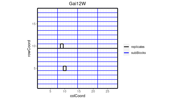

Note that the default title of the plot is the name of the trial. This can be manually changed using the title argument.

This plot can be extended by highlighting interesting genotypes in the layout. By default the default ggplot2 package colors are used for highlighting these genotypes. Custom colors can be specified using the colHighlight argument.

## Plot the layout for Gai12W.
## Highlight genotypes A3 and 11430 in red and blue.
plot(dropsTD, 
     trials = "Gai12W", 
     highlight = c("A3", "11430"),
     colHighlight = c("red", "blue"))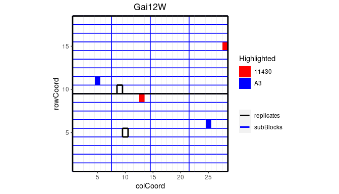

It is also possible to color the sub blocks within the field. By default the default ggplot2 package colors are used for coloring these sub blocks. Custom colors can be specified using the colSubBlock argument.

## Plot the layout for Gai12W.
## Color sub blocks using polychrome colors for high contrast.
## Colors are specified here since this color palette is only available as such
## from R > 4.0.
cols <- c("#5A5156", "#E4E1E3", "#F6222E", "#FE00FA", "#16FF32", "#3283FE", 
          "#FEAF16", "#B00068", "#1CFFCE", "#90AD1C", "#2ED9FF", "#DEA0FD", 
          "#AA0DFE", "#F8A19F", "#325A9B", "#C4451C", "#1C8356", "#85660D", 
          "#B10DA1", "#FBE426", "#1CBE4F", "#FA0087", "#FC1CBF", "#F7E1A0", 
          "#C075A6", "#782AB6", "#AAF400", "#BDCDFF", "#822E1C", "#B5EFB5", 
          "#7ED7D1", "#1C7F93", "#D85FF7", "#683B79", "#66B0FF", "#3B00FB")
plot(dropsTD, 
     trials = "Gai12W", 
     colorSubBlock = TRUE,
     colSubBlock = cols)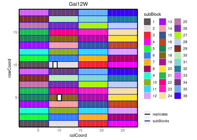

Highlighting genotypes and coloring subBlocks cannot be done simultaneously. If both options are specified, only highlighting is done.

It is possible to add the labels of the genotypes to the layout.

## Plot the layout for Gai12W, label the genotypes.
plot(dropsTD, 
     trials = "Gai12W", 
     showGeno = TRUE)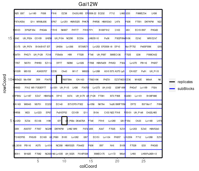

We can visualize the raw data of a given trait on the layout, as a heatmap. This type of plot gives a first indication of the spatial variability for a given trial. This can be further investigated with the spatial modeling. Missing plots are shown in white.

## Plot the layout for Gai12W, show raw data for grain yield.
plot(dropsTD, 
     trials = "Gai12W", 
     traits = "grain.yield")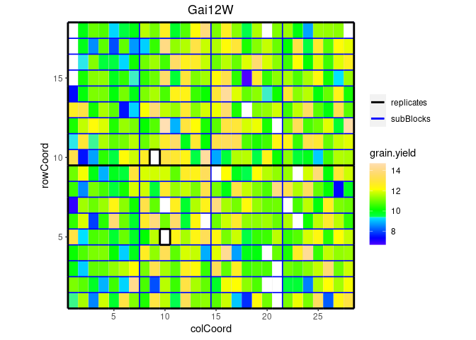

Map plot

A second type of plot displays the trial locations on a map. This plot is made based on trLat and trLong in the metadata. If latitude or longitude is not available for a certain location, then this location is not plotted. If the locations are very close to one another, the resulting map can become quite small. The arguments minLatRange and minLongRange can be used to extend the minimum range of latitude and longitude respectively to address this issue. For map plots, where there are many trials close to one another, the trial names can be left out of the plot by specifying the argument printTrialNames = FALSE.

## Plot the locations of the trials on a map.
plot(dropsTD, 
     plotType = "map")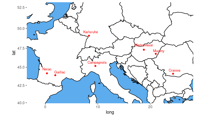

It is possible to color the trials by a variable in the TD object using the argument colorTrialBy. Colors can be specified with the argument colTrial.

## Plot the locations of the trials on a map.
## Color the trials by water scenario.
plot(dropsTD, 
     plotType = "map",
     colorTrialBy = "scenarioWater",
     colTrial = c("red", "darkgreen"))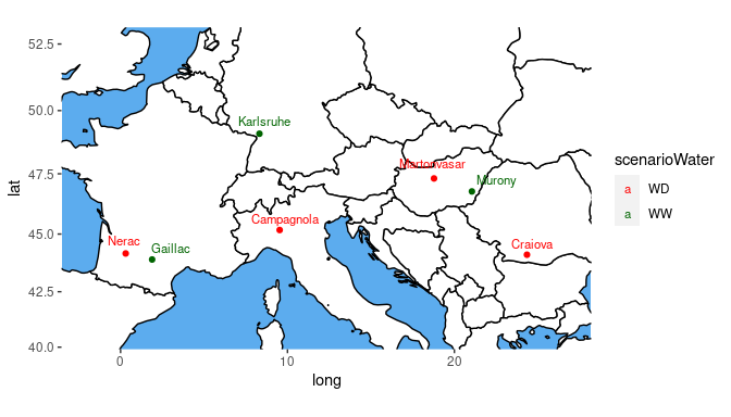

Box plot

Boxplots can be made to get an idea of the contents of the data in the TD object. By default a box is plotted per trial in the data for the specified traits. Boxplots for multiple traits can be made at once.

Boxplots can be made to visually assess the variability of the trait(s) in the TD object. By default a box is plotted per trial for the specified trait. Boxplots for multiple traits can be made at once.

## Create a boxplot for grain yield.
plot(dropsTD, 
     plotType = "box", 
     traits = "grain.yield")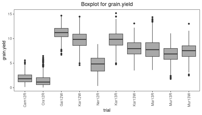

The trials in the box plot can be grouped by using the argument groupBy. Colors can be applied to groups within trials by specifying the argument colorTrialBy. As in other plots the argument colTrial can be used to specify the colors used. The boxes for the (groups of) trials can be ordered using the argument orderBy. Boxes can be ordered alphabetically (orderBy = "alphabetic"), and by ascending (orderBy = "ascending") and descending (orderBy = "descending") trait mean.

## Create a boxplot for grain yield with boxes grouped by year 
## Color the boxes by scenario within years.
plot(dropsTD, 
     plotType = "box", 
     traits = "grain.yield", 
     groupBy = "year", 
     colorTrialBy = "scenarioFull")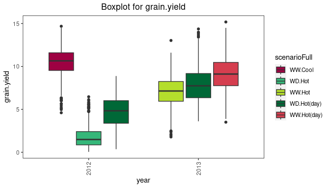

Correlation plot

Another plot, that can be made, is a plot of the correlations between the trials for a specified trait. The order of the plotted trials is determined by clustering them and plotting closely related trials close to one another.

## Create a correlation plot for grain yield.
plot(dropsTD, 
     plotType = "cor", 
     traits = "grain.yield")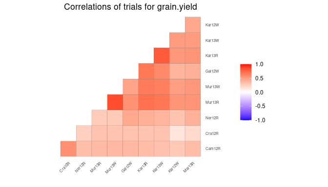

Scatter plot matrix

Finally a scatter plot matrix can be made. The lower triangular of the matrix displays scatter plots between trials. The diagonal of the scatter plot matrix visualizes histograms of the data per trial. It is possible to calculate the correlation between trials and print them in the scatter plots by specifying the addCorr argument. The addCorr argument can take the values "tl" (top left), "tr" (top right), "bl" (bottom left) or "br" (bottom right). This indicates, where the correlation is placed in each of the scatter plots. It is possible to color the genotypes and trials in the plots by a variable in the TD object by specifying the arguments colorTrialBy, and colorGenoBy, respectively.

## Create a scatter plot matrix for grain yield.
## Color trials by scenario and genotypes by family.
plot(dropsTD, 
     plotType = "scatter", 
     traits = "grain.yield", 
     colorTrialBy = "scenarioFull", 
     colorGenoBy = "geneticGroup")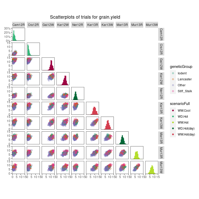

Modeling

To get genotypic predictions we want to accurately separate the genetic effects from the spatial effects and further design factors. To do this, for each trial a model can be fitted for the trait we are interested in. In the statgenSTA package models can be fitted using functions from the packages SpATS (Rodríguez-Álvarez et al. 2018), lme4 (Bates et al. 2015), or ASReml (Butler et al. 2017). For models with row column or resolvable row column design, "SpATS" is the default engine, for the other models "lme4" is used by default. This can always be overruled by specifying the function argument engine.

Models can be fitted on the trial data in a TD object using the function fitTD(). The exact model fitted depends on the design of the trial (see Model types). The design can be specified by a function argument or included in the metadata of the TD object as described in Metadata. In the former case, the same model will be fitted for all trials, in the latter, different models can be fitted for different trials. If both are available the function argument will always be leading.

The output of the fitTD() function is an object of class STA (Single Trial Analysis), a list of fitted models with one element for each trial the model was fitted for.

Model types

Models can be fitted for five different trial designs. These are listed in the following table with their respective model specifications.

design	code	model fitted
incomplete block design	`"ibd"`	trait = subBlock + genotype + \(\epsilon\)
resolvable incomplete block design	`"res.ibd"`	trait = repId + repId:subBlock + genotype + \(\epsilon\)
randomized complete block design	`"rcbd"`	trait = repId + genotype + \(\epsilon\)
row column design	`"rowcol"`	trait = rowId + colId + genotype + \(\epsilon\)
resolvable row column design	`"res.rowcol"`	trait = repId + repId:rowId + repId:colId + genotype + \(\epsilon\)

In the models above, fixed effects are indicated in italics, whereas random effects are indicated in bold. The term genotype can be fitted as fixed or as random effect depending on the value of the argument what. Extra fixed effects may be fitted using the argument covariates.
If "SpATS" is used as modeling engine, an extra spatial term is always included in the model (see Spatial models). A spatial term is also included when the modeling engine is "asreml" and the function argument spatial is set to TRUE.

Using the TD object named dropsTD from the previous section, a model for the trial Gai12W and trait grain.yield can now be fitted on the data. The trial was set up using a resolvable row column design. This is specified in fitTD() using the argument design. Since engine is not specified as an argument, "SpATS" is used as engine for fitting the model.

## Fit a single trial model using a model based on a resolvable row column design.
modDropsSp <- fitTD(TD = dropsTD, 
                    trials = "Gai12W", 
                    traits = "grain.yield",
                    design = "res.rowcol")

Note that by not supplying the what argument in the fitTD() function, two models are fitted. One for genotype as a fixed effect and one for genotype as a random effect. The results of both these models are stored in the STA object named modDropsSp. This is very useful for extracting different results from the model later on. A trade-off is that fitting two models takes more time than fitting only one. Therefore, when fitting models to large data sets it is sensible to explicitly define the what argument if only a specific subset of the results is needed as output.

## Fit a single trial model with genotype as random effect.
modDropsSp2 <- fitTD(TD = dropsTD, 
                     trials = "Gai12W", 
                     traits = "grain.yield", 
                     what = "random", 
                     design = "res.rowcol")

Spatial models

When using "SpATS" as a modeling engine for fitting a model, an extra spatial component is always included in the model. This spatial component is composed using the PSANOVA() function in the SpATS package, which uses 2-dimensional smoothing with P-splines as described in Lee, Durbán, and Eilers (2013) and in Rodríguez-Álvarez et al. (2018). See help(PSANOVA, SpATS) for a detailed description. The arguments nseg and nest.div of the PSANOVA() function can be modified using the control argument in the fitTD() function.
The default number for the number of segments is (number of columns / 2, number of rows / 2). Fitting the model in the previous section specifying the number of segments for columns and rows as 28 and 18 respectively, works as follows:

## Fit a spatial single trial model using SpATS. 
## Manually specify the number of segments for rows and columns.
modDropsSp3 <- fitTD(TD = dropsTD, 
                     trials = "Gai12W", 
                     traits = "grain.yield", 
                     design = "res.rowcol", 
                     control = list(nSeg = c(28, 18)))

Alternatively, spatial models can be fitted using "asreml" as modeling engine and setting the argument spatial = TRUE. In this case seven models are fitted and the best model, based on a goodness-of-fit criterion, either AIC or BIC. The default is AIC, this can be modified with the control argument in the fitTD() function.

The seven models fitted largely depend on the trial design. On top of the model described in the previous section extra random terms are added. These extra random terms depend on the structure of the data. If the trial has a regular structure, i.e. all replicates appear the same amount of times in the trial, the following combinations of random and spatial terms are fitted:

Random part	Spatial part
random effects based on design	none
random effects based on design	AR1(rowId):colId
random effects based on design	rowId:AR1(colId)
random effects based on design	AR1(rowId):AR1(colId)
random effects based on design + nugget	AR1(rowId):colId
random effects based on design + nugget	rowId:AR1(colId)
random effects based on design + nugget	AR1(rowId):AR1(colId)

If the design is not regular the following combinations of random and spatial terms are fitted:

Random part	Spatial part
random effects based on design	none
random effects based on design	exp(rowCoord):colCoord
random effects based on design	rowCoord:exp(colCoord)
random effects based on design	iexp(rowCoord, colCoord)
random effects based on design + nugget	exp(rowCoord):colCoord
random effects based on design + nugget	rowCoord:exp(colCoord)
random effects based on design + nugget	iexp(rowCoord,colCoord)

Fitting a model similar to the one above using asreml with BIC as goodness-of-fit criterion works as follows:

if (requireNamespace("asreml", quietly = TRUE)) {
  ## Fit a spatial single trial model using asreml.
  modDropsAs <- fitTD(TD = dropsTD, 
                      trials = "Gai12W", 
                      traits = "grain.yield", 
                      design = "res.rowcol", 
                      spatial = TRUE, 
                      engine = "asreml",
                      control = list(criterion = "BIC"))
}

The fitted models and the best model are stored in the output together with a summary table with details on the fitted models.

if (exists("modDropsAs")) {
  ## Overview of fitted models.
  print(modDropsAs$Gai12W$sumTab$grain.yield, digits = 2, row.names = FALSE)
}

Model summary

Since genotype has been fitted both as fixed and as random factor in the object named modDropsSp, it is possible to calculate both the Best Linear Unbiased Estimators (BLUEs) and the Best Linear Unbiased Predictors (BLUPs). Therefore, both are printed in the summary of the model together with their respective standard errors.

## Set nBest to 5 to limit the output to the best 5 genotypes.
summary(modDropsSp, 
        nBest = 5)
#> Summary statistics 
#> ==================
#> 
#> Summary statistics for grain.yield in Gai12W  
#> 
#>                          grain.yield
#> Number of observations         483.0
#> Number of missing values        19.0
#> Mean                           11.23
#> Median                         11.22
#> Min                             6.71
#> Max                            14.68
#> First quantile                 10.38
#> Third quantile                 12.09
#> Variance                       1.845
#> 
#> 
#> Estimated heritability 
#> ======================
#> 
#> Heritability: 0.84 
#> 
#> Predicted means (BLUEs & BLUPs) 
#> ===============================
#> Best 5 genotypes
#>            BLUEs       SE    BLUPs     SE
#> Lo1261  13.98285  0.47144 13.65848 0.4329
#> Lo1253  13.88760  0.47244 13.44540 0.4350
#> Lo1223  13.71634  0.47173 13.28001 0.4337
#> DKMBST  13.63513  0.47242 13.23844 0.4345
#> HMV5422 13.56305  0.68282 13.02194 0.5785

Model plots

Two types of plots can be made for fitted model objects of class STA.

Base plots

The first is a series of four plots, a histogram of the residuals, a normal quantile plot of the residuals, a scatter plot of residuals against fitted values and a scatter plot of absolute residuals against fitted values. These plots can be made by calling plot() on the STA object. Plots can be made for multiple trials and multiple traits simultaneously, either for the model with genotype as fixed effect or for the model with genotype as random effect. By default plots are made for all trials and all traits, but this can be restricted using the arguments trials and traits. If only one model is fitted the results of the fitted model will be plotted. In case both models were fitted, as a default the results will be plotted for the model with genotype fixed. This can be changed using the argument what.

## Base plots for the model with genotype fitted as random effect.
plot(modDropsSp, 
     plotType = "base", 
     what = "random")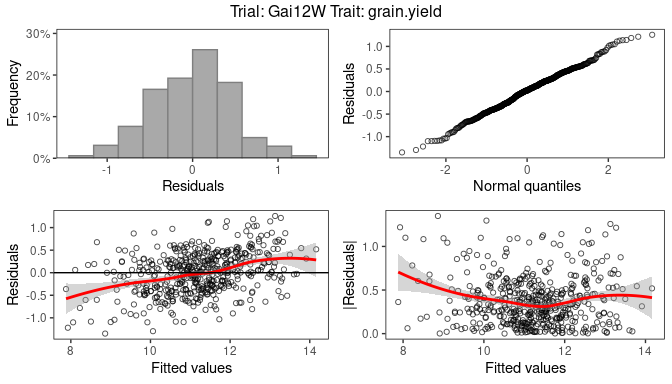

Spatial plots

The second type of plot consists of five plots, spatial plots of the raw data, fitted values, residuals and either BLUEs or BLUPs, and a histogram of the BLUEs or BLUPs. If "SpATS" was used as engine for modeling an extra plot with the fitted spatial trend is included. The spatial trend can be displayed on the original scale (default, spaTrend = "raw") or as percentage (spaTrend = "percentage"). In the latter case the spatial trend is scaled (i.e., divided by the average of the observed response variable of interest across the field) and displayed as percentage. The call for creating these plots is similar to the base plots, but requires the specification of the argument plotType = "spatial". Note that spatial plots can only be made if spatial information, i.e. rowCoord and colCoord, is available in the TD object.

## Spatial plot for the model with genotype fitted as fixed effect.
plot(modDropsSp, 
     plotType = "spatial")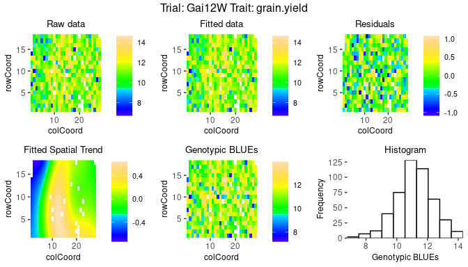

## Spatial plot for the model with genotype fitted as fixed effect.
## Display the spatial trend as a percentage.
plot(modDropsSp, 
     plotType = "spatial", 
     spaTrend = "percentage")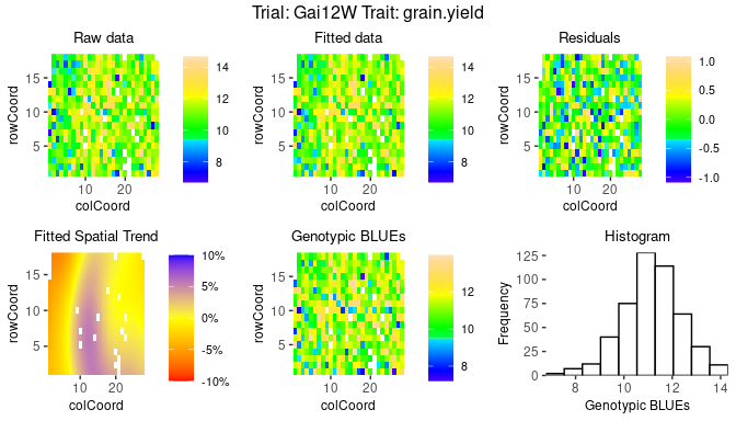

Outlier detection

After fitting a model, it is possible to perform an outlier detection on the results. This outlier detection checks the residuals in the fitted model and compares them to a limit. Observations with a residual larger than this limit are marked as outliers. The default limit is calculated based on the number of observations in the data. Setting a custom limit is also possible.

## Outlier detection for the model with genotype fitted as random.
outliers <- outlierSTA(modDropsSp, 
                       traits = "grain.yield",
                       what = "random")
#> No large standardized residuals.

The output of the outlier detection function is a data.frame with the outliers and of vector of indices of the outliers in the original data. This vector can be used for removing outliers from the data.

It is possible to perform outlier detection on a model with genotype fitted as fixed, however, in doing so it is only possible to detect outliers in genotypes that are replicated in the data. For unreplicated genotypes the residual will always be 0 and, therefore, these genotypes will never be marked as outliers.

To get an idea of the magnitude of the outliers, the argument commonFactors can be used to see the values of observations with similar characteristics. In the example below, for all outliers also the other observations for the same genotype are shown.

## Outlier detection for the model with genotype fitted as random.
## A custom limit is used and commonFactors set to genotype.
outliers <- outlierSTA(modDropsSp, 
                       traits = "grain.yield", 
                       what = "random",
                       rLimit = 2.7, 
                       commonFactors = "genotype")
#> Large standardized residuals.
#> 
#>   trial genotype       trait     value       res outlier
#>  Gai12W     A347 grain.yield  8.767218 -2.766018    TRUE
#>  Gai12W     A347 grain.yield 10.448529  1.853837   FALSE
#>  Gai12W     B105 grain.yield  7.513174 -2.875952    TRUE
#>  Gai12W     B105 grain.yield  9.331618  1.438732   FALSE

Model reports

For objects of class STA there is a report() function available in the statgenSTA package. This function creates a pdf report summarizing the main results of the fitted model. Also, the tex file and figures used for generating the pdf report are saved. By editing the tex file it is possible to modify the report to one’s needs, providing high flexibility.

When no outfile is specified, reports will be created with a default names, e.g. “modelReport_trial_trait_fixed_timestamp.pdf”, in the current working directory. The argument outfile can be used to change the name and location of the report. The value of this argument should be a valid location and name for a pdf file, i.e. including the postfix “.pdf”. Non-existing directories are created by the report() function. When an outfile is specified, trial, trait and modeltype (fixed or random) are concatenated to it in the name of the report.

The reports contain general information on the model fitted, a summary of the results, the plots described in the previous section, a list of best (highest BLUEs or BLUPs) genotypes and a scatter plot of all genotypes and their BLUEs or BLUPs. For some traits a low value might mean a genotype is performing well. To correctly show the best genotypes in the report in this case, set the argument descending to TRUE in the report() function.

## Create a report in the current working directory
report(modDropsSp)
## Create a report for the model with genotype fitted as random.
report(modDropsSp, 
       outfile = "./myReports/dropsReport.pdf", 
       what = "random")

Reporting for an object of class STA can be done for multiple trials, traits and model types simultaneously. For each combination of trial, trait and model type, a separate pdf report will be created. The arguments traits, trials and what can be used for specifying the models for which the reports should be generated.

Extracting model results

After fitting a model, various results can be extracted or calculated from the fitted model using the function extractSTA(). This can be anything from a single result for one trait and one trial to a list of different results for all models in an object of class STA. The results, which can be extracted, depend on the type of model fitted and sometimes on the modeling engine as well. For example, BLUEs can only extracted if genotype was fitted as a fixed effect. On the other hand, BLUPs and heritabilities can only be calculated and extracted if genotype was fitted as random effect.

All results, that can be extracted, are shown in the table below. In the first column is the result. This is also the value to be used for the argument what in order to extract the corresponding result with the extractSTA() function. The second column shows what model needs to be fitted in order to be able to extract the result. Here F denotes genotype as fixed effect, and R genotype as random effect. The third column gives a short description of the result that will be extracted and, where needed, also states for which modeling engines it can be extracted. The final columns shows, whether the result can be extracted as a data.frame or not. Results that cannot be extracted as a data.frame will be extracted as a list. E.g. BLUES by default will be extracted in a data.frame and varCompF as a list. When extracting multiple results at once, the result will always be a list. E.g., when extracting BLUEs and BLUPs the result we be a list with two items per trial, named BLUEs and BLUPs.

result	model	description	asDataFrame
BLUEs	F	Best Linear Unbiased Estimators	yes
seBLUEs	F	standard errors of the BLUEs	yes
ue	F	unit errors - only for lme4 and asreml	yes
varCompF	F	variance components for the model with genotype as fixed component
fitted	F	fitted values for the model with genotype as fixed component	yes
residF	F	residuals for the model with genotype as fixed component	yes
stdResF	F	standardized residuals for the model with genotype as fixed component	yes
wald	F	results of the wald test - only for lme4 and asreml
CV	F	Coefficient of Variation	yes
rDfF	F	residual degrees of freedom for the model with genotype as fixed component	yes
sed	F	standard error of difference - only for asreml
lsd	F	least significant difference - only for asreml
BLUPs	R	Best Linear Unbiased Predictors	yes
seBLUPs	R	standard errors of the BLUPs	yes
heritability	R	generalized heritability	yes
varCompR	R	variance components for the model with genotype as random component
varGen	R	genetic variance component	yes
varErr	R	residual variance component	yes
varSpat	R	spatial variance components - only for SpATS
rMeans	R	fitted values for the model with genotype as random component	yes
ranEf	R	random genetic effects	yes
residR	R	residuals for the model with genotype as random component	yes
stdResR	R	standardized residuals for the model with genotype as random component	yes
rDfR	R	residual degrees of freedom for the model with genotype as random component	yes
effDim	R	effective dimensions - only for SpATS
ratEffDim	R	ratios of the effective dimensions - only for SpATS

Note that when predictions are made (e.g. when extracting BLUEs, BLUPs or their standard errors), those predictions are always obtained by averaging over all levels of the fixed factors in the model.

Using the argument what = "all" in the extractSTA() function call, extracts all results possible for the fitted model. This is also the default.

Below are some examples of extracting results from a fitted model. Recall that modDropsSp contains two fitted models, one with genotype as fixed effect and one with genotype as random effect.

## Extract BLUEs.
BLUEsDrops <- extractSTA(STA = modDropsSp, 
                         what = "BLUEs")
## Extract BLUEs and BLUPs.
predDrops <- extractSTA(STA = modDropsSp, 
                        what = c("BLUEs", "BLUPs"))

Note that BLUEsDrops is a data.frame, whereas predDrops is a list with one item, since we fitted a model for only one trial.

Adding extra variables

The data.frame named BLUEsDrops consists of only three columns: genotype, trial, and grain.yield. If the model would have been fitted for multiple traits all these traits would become columns in the data.frame. It might be useful to add extra columns from the data used to fit the model to the output for use in further analysis of the data. This can be achieved using the argument keep in the extractSTA() function. To include the water scenario in the output, useful for using the BLUEs for a GxE analysis, use the following command:

## Extract BLUEs from the fitted model.
BLUEsDrops2 <- extractSTA(STA = modDropsSp, 
                          what = "BLUEs", 
                          keep = "scenarioWater")
head(BLUEsDrops2)
#>   genotype  trial scenarioWater grain.yield
#> 1    11430 Gai12W            WW   11.707337
#> 2       A3 Gai12W            WW   11.564098
#> 3     A310 Gai12W            WW   11.056274
#> 4     A347 Gai12W            WW    9.499485
#> 5     A374 Gai12W            WW   10.954845
#> 6     A375 Gai12W            WW   10.808332

Multiple columns can be included in the output in this way. Note that not every column from the original TD object can be included in the extracted data. Only columns that, for each genotype, have only one value per trial can be included. For example, the column repId containing replicates, that has several different values for a single genotype within each trial, cannot be included. When trying to do so it will be ignored with a warning.
It is, however, possible to include repId when extracting fitted values, since for each observation in the original data a fitted value is computed.

## Extract fitted values from the model.
## Add repId and family to the output.
fitVals <- extractSTA(STA = modDropsSp, 
                      what = "fitted", 
                      keep = c("repId", "geneticGroup"))
head(fitVals)
#>   genotype  trial repId geneticGroup grain.yield
#> 1    DE811 Gai12W     1  Stiff_Stalk    9.767671
#> 2  UH_P089 Gai12W     1       Iodent   11.133769
#> 3    W182E Gai12W     1        Other    8.929808
#> 4      Lp5 Gai12W     1  Stiff_Stalk   11.967323
#> 5    F7082 Gai12W     1        Other    8.921387
#> 6   Lo1087 Gai12W     1  Stiff_Stalk   13.213437

Prepare data for GxE analysis

Performing a GxE analysis on can be done using the statgenGxE package. This package uses the same input format for its analyses as the statgenSTA package.

To use the BLUEs or BLUPs from the fitted model in a GxE analysis they can easily be converted into a TD object using the function STAtoTD(). This function creates a TD object from a fitted model including one or more of the following: BLUEs, standard errors of BLUEs, BLUPs and standard errors of BLUPs. Optionally, a column wt with weights (calculated as \((1 / seBLUEs)^2\)) can be added as well. In the same way as described in the previous section extra columns can be added to the output using the argument keep.

## Fit a model for all trials with genotype as fixed factor.
modDropsSpTot <- fitTD(TD = dropsTD, 
                       traits = "grain.yield", 
                       what = "fixed", 
                       design = "res.rowcol")
## Create a TD object containing BLUEs and standard errors of BLUEs.
TDGxE <- STAtoTD(STA = modDropsSpTot, 
                 what = c("BLUEs", "seBLUEs"))
## Add weights and water scenario to the output.
TDGxE2 <- STAtoTD(STA = modDropsSpTot, 
                  what = c("BLUEs", "seBLUEs"), 
                  keep = "scenarioWater",
                  addWt = TRUE)

References

Bates, Douglas, Martin Mächler, Ben Bolker, and Steve Walker. 2015. “Fitting Linear Mixed-Effects Models Using Lme4.” Journal of Statistical Software 67 (1). https://doi.org/10.18637/jss.v067.i01.

Butler, D. G., B. R. Cullis, A. R. Gilmour, B. G. Gogel, and R. Thompson. 2017. “ASReml-r Reference Manual Version 4.” https://vsni.co.uk/.

Lee, Dae-Jin, María Durbán, and Paul Eilers. 2013. “Efficient Two-Dimensional Smoothing with p-Spline ANOVA Mixed Models and Nested Bases.” Computational Statistics & Data Analysis 61 (May): 22–37. https://doi.org/10.1016/j.csda.2012.11.013.

Millet, Emilie J., Cyril Pommier, Mélanie Buy, Axel Nagel, Willem Kruijer, Therese Welz-Bolduan, Jeremy Lopez, et al. 2019. “A Multi-Site Experiment in a Network of European Fields for Assessing the Maize Yield Response to Environmental Scenarios.” Portail Data Inra. https://doi.org/10.15454/IASSTN.

Millet, Emilie, Claude Welcker, Willem Kruijer, Sandra Negro, Stephane Nicolas, Sebastien Praud, Nicolas Ranc, et al. 2016. “Genome-Wide Analysis of Yield in Europe: Allelic Effects as Functions of Drought and Heat Scenarios.” Plant Physiology, July, pp.00621.2016. https://doi.org/10.1104/pp.16.00621.

Rodríguez-Álvarez, María, Martin P. Boer, Fred van Eeuwijk, and Paul H. C. Eilers. 2018. “Correcting for Spatial Heterogeneity in Plant Breeding Experiments with p-Splines.” Spatial Statistics 23 (October): 52–71. https://doi.org/10.1016/j.spasta.2017.10.003.

Bart-Jan van Rossum

2024-10-14

The statgenSTA Package

Data preparation

Creating a `TD` object

Example

Metadata

Add extra data to a `TD` object

Summarizing a `TD` object

Plotting a `TD` object

Layout plot

Map plot

Box plot

Correlation plot

Scatter plot matrix

Modeling

Model types

Spatial models

Model summary

Model plots

Base plots

Spatial plots

Outlier detection

Model reports

Extracting model results

Adding extra variables

Prepare data for GxE analysis

References

Modeling field trials using statgenSTA

Bart-Jan van Rossum

2024-10-14

The statgenSTA Package

Data preparation

Creating a TD object

Example

Metadata

Add extra data to a TD object

Summarizing a TD object

Plotting a TD object

Layout plot

Map plot

Box plot

Correlation plot

Scatter plot matrix

Modeling

Model types

Spatial models

Model summary

Model plots

Base plots

Spatial plots

Outlier detection

Model reports

Extracting model results

Adding extra variables

Prepare data for GxE analysis

References

Creating a `TD` object

Add extra data to a `TD` object

Summarizing a `TD` object

Plotting a `TD` object