statgenHTP tutorial: 5. Modelling the temporal evolution of the genetic signal

Diana M. Pérez-Valencia, María Xosé Rodríguez-Álvarez, Bart-Jan van Rossum, Emilie Millet, Martin Boer, Fred van Eeuwijk

2022-12-13

Introduction

This document presents the second stage of the two-stage approach proposed by Pérez-Valencia et al. (2022). The aim is modeling the temporal evolution of the genetic signal after a spatial correction is performed on a phenotypic trait (see statgenHTP tutorial: 3. Correction for spatial trends).

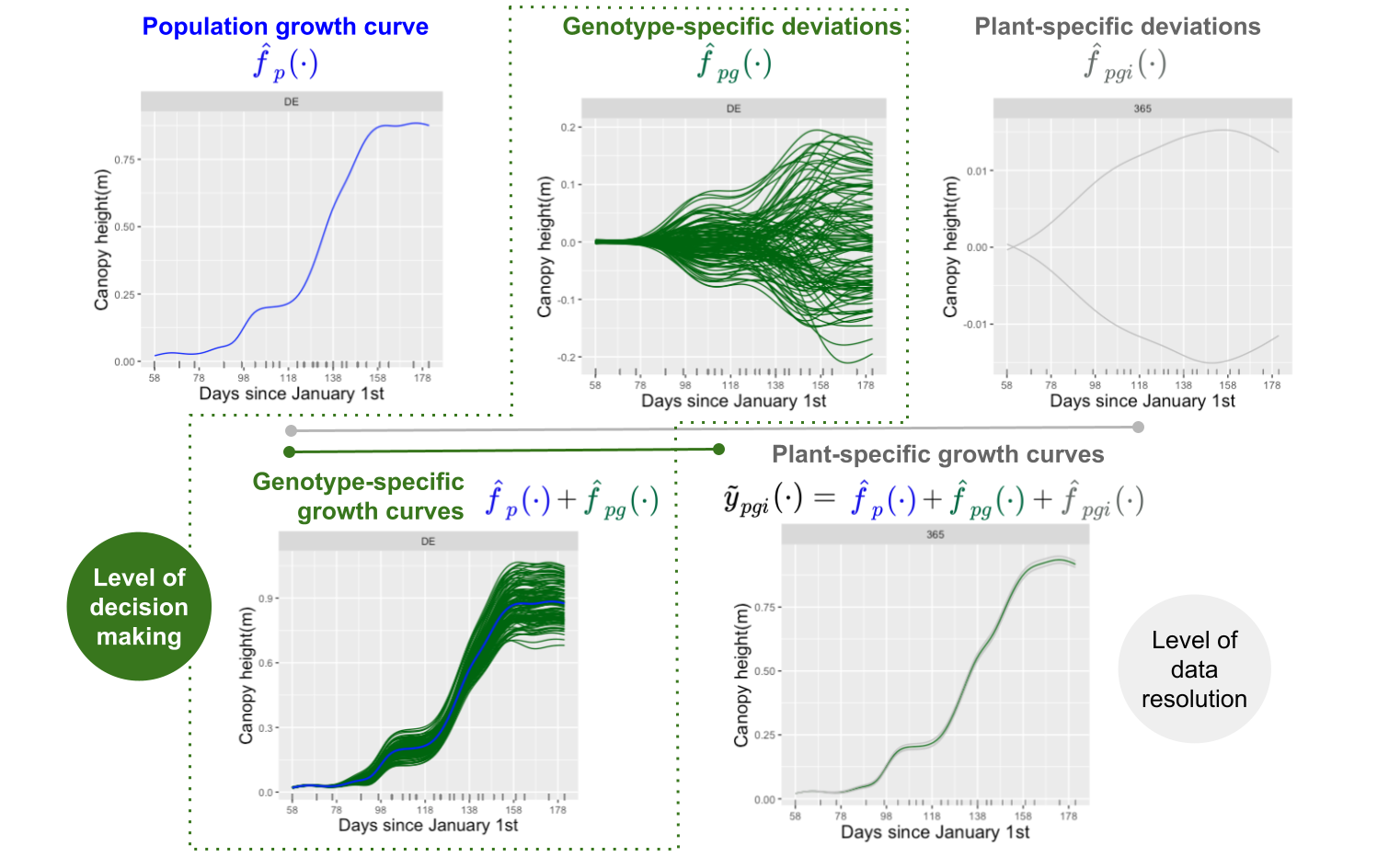
Data consist of time-series (curves) of a (possibly) spatially corrected plant/plot phenotype. We assume that data present a hierarchical structure with plots nested in genotypes, and genotypes nested in “populations”. We denote as \(\tilde{y}_{pgi}(t)\) the spatially corrected phenotype for the \(i\)th plant (\(i = 1,\ldots,m_{pg}\)) of the \(g\)th genotype \(g=1,\ldots,\ell_p\) in the \(p\)th population (\(p= 1,\ldots, k\)) at time \(t\). As such, there is a total of \(M=\sum_{p=1}^k{\sum_{g=1}^{\ell_p}{m_{pg}}}\) plots/plants, \(L=\sum_{p=1}^k{\ell_p}\) genotypes, and \(k\) populations. To model this sample of curves the following additive decomposition of the phenotypic variation over time is considered, and a P-spline-based three-level nested hierarchical data model (hereafter refer as psHDM) is used

\(\tilde{y}_{pgi}(t) = f_{p}(t) + f_{pg}(t) + f_{pgi}(t) + \varepsilon_{pgi}(t),\;\;\varepsilon_{pgi}(t)\sim N\left(0, \sigma^{2}w_{pgi}(t)\right),\)

where

• \(f_{p}\) is the \(p\)th population mean function.
• \(f_{pg}\) is the genotype-specific deviation from \(f_p\) for the \(g\)th genotype. Note that \(f_{p} + f_{pg}\) represents the genotype-specific trajectory for the \(g\)th genotype.
• \(f_{pgi}\) is the plot-specific deviation from \(f_{pg}\) for the \(i\)th plot. In the same way than for the genotypes, \(f_{p} + f_{pg} + f_{pgi}\) is the plot-specific trajectory for the \(i\)th plot.
• \(\varepsilon_{pgi}\) is the random noise curve, and \(w_{pgi}\) is the weight obtained from, e.g., the spatial correction.

An illustration of these curves follows

Before proceeding, we note that the functions described in this tutorial can be applied to both spatially corrected data (see statgenHTP tutorial: 3. Correction for spatial trends) or raw data. These functions also allow estimating first- and second-order derivative curves from trajectory and deviation curves at the three levels of the hierarchy (populations, genotypes and plots/plants). All these curves can be used as input to extract time‐independent parameters to characterise genotypes (see statgenHTP tutorial: 6. Estimation of parameters from time courses).

To illustrate the analysis, we use the maize data corrected for spatial trends, spatCorrectedArch. The data structure is as follows

data(spatCorrectedArch)
str(spatCorrectedArch)
#> 'data.frame':    40573 obs. of  10 variables:
#>  $ timeNumber   : int  1 1 1 1 1 1 1 1 1 1 ...
#>  $ timePoint    : POSIXct, format: "2017-04-13" "2017-04-13" ...
#>  $ LeafArea_corr: num  0.00256 0.0024 0.00321 0.00303 0.00269 ...
#>  $ LeafArea     : num  0.00287 0.00252 0.00338 0.00326 0.00249 ...
#>  $ wt           : num  2262 2262 2262 2262 2262 ...
#>  $ genotype     : Factor w/ 90 levels "GenoA01","GenoA02",..: 1 1 1 1 1 2 2 2 2 2 ...
#>  $ geno.decomp  : Factor w/ 4 levels "WD_Panel1","WD_Panel2",..: 1 1 1 1 1 1 1 1 1 1 ...
#>  $ rowId        : int  2 3 26 24 56 38 60 16 24 52 ...
#>  $ colId        : int  16 28 24 20 21 16 20 24 21 28 ...
#>  $ plotId       : Factor w/ 1673 levels "c10r1","c10r10",..: 368 1156 914 672 767 388 712 903 732 1181 ...

For this specific example we first need to specify the genotype-by-treatment interaction (genotype-by-water regime). As is explained in Pérez-Valencia et al. (2022), the actual implementation of the psHDM model does not allow for crossed effect, but only for nested effects. As such, to analyse this dataset with the proposed model, we combine the genotype and the water regime information as follows (i.e., \(180\) genoTreat = \(90\) genotype \(\times\) \(2\) treat)

str(spatCorrectedArch[["geno.decomp"]])
#>  Factor w/ 4 levels "WD_Panel1","WD_Panel2",..: 1 1 1 1 1 1 1 1 1 1 ...
str(spatCorrectedArch[["genotype"]])
#>  Factor w/ 90 levels "GenoA01","GenoA02",..: 1 1 1 1 1 2 2 2 2 2 ...

## Extracting the treatment: water regime (WW, WD).
spatCorrectedArch[["treat"]] <- as.factor(substr(spatCorrectedArch[["geno.decomp"]],
                                                 start = 1, stop = 2))
str(spatCorrectedArch[["treat"]])
#>  Factor w/ 2 levels "WD","WW": 1 1 1 1 1 1 1 1 1 1 ...

## Specifying the genotype-by-treatment interaction.
spatCorrectedArch[["genoTreat"]] <-
  interaction(spatCorrectedArch[["genotype"]],
             spatCorrectedArch[["treat"]], sep = "_")

str(spatCorrectedArch[["genoTreat"]])
#>  Factor w/ 180 levels "GenoA01_WD","GenoA02_WD",..: 1 1 1 1 1 2 2 2 2 2 ...

We will use the spatially corrected leaf area (LeafArea_corr) as response variable. We assume that plots (plotId, \(M = 1673\)) are nested in genotype-by-water regime (genoTreat, \(L = 180\)), and genotype-by-water regime are nested in populations/panel-by-water regime (geno.decomp, \(k = 4\)). Furthermore, uncertainty is propagated from stage to stage using weights (wt). Since we are in the context of longitudinal models, it is natural that we use time as a covariate (i.e., the timepoints at which the phenotype of interest was measured). We note that the implemented function requires numerical times. If the timeNumber column is used as it is returned by the getCorrected() function, the user has to be aware that it is a simple enumeration of the timepoints. Care must be taken when dealing with non-equidistant timepoints to keep the same time scale as in the original timePoint column. The user can also specify any other numerical time transformation. For instance, in this example, we first construct a new column called DOY with time in days of the year

## Create a new timeNumber with days of the year (DOY)
spatCorrectedArch[["DOY"]] <- as.numeric(strftime(spatCorrectedArch$timePoint, format = "%j"))

The following code depicts the kind of curves that are modelled here (at plant/plot level)

ggplot2::ggplot(data = spatCorrectedArch,
                ggplot2::aes(x= DOY, y = LeafArea_corr, group = plotId)) +
  ggplot2::geom_line(na.rm = TRUE) +
  ggplot2::facet_grid(~geno.decomp) +
  ggplot2::labs(y = "Spatially corrected leaf area")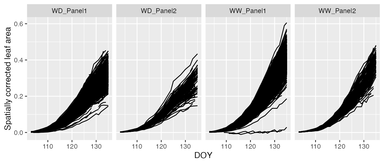

---

Fit the P-spline Hierarchical Curve Data Model (psHDM)

To fit the psHDM model, we use the fitSplineHDM() function (results of the fitting process are provided below)

## Fit P-Splines Hierarchical Curve Data Model for all genotypes.
fit.psHDM  <- fitSplineHDM(inDat = spatCorrectedArch,
                           trait = "LeafArea_corr",
                           useTimeNumber = TRUE,
                           timeNumber = "DOY",
                           pop = "geno.decomp",
                           genotype = "genoTreat",
                           plotId = "plotId",
                           weights = "wt",
                           difVar = list(geno = FALSE, plot = FALSE),
                           smoothPop = list(nseg = 7, bdeg = 3, pord = 2),
                           smoothGeno = list(nseg = 7, bdeg = 3, pord = 2),
                           smoothPlot = list(nseg = 7, bdeg = 3, pord = 2),
                           trace = TRUE)

In the example above, we use cubic (\(bdeg = 3\)) B-spline basis of dimension \(b_{pop} = b_{gen} = b_{plot} = 10\) and second order penalties (\(pord = 2\)) to represent \(f_p\), \(f_{pg}\) and \(f_{pgi}\). We note that the fitSplineHDM() function uses as argument the number of segments nseg instead of the number of B-spline basis \(b\) (nseg = \(b\) - bdeg, that is, for our example, if \(b = 10\) then nseg = 7). We encourage the user to try different values for nseg and compare the results. Under this model configuration, the mixed model formulation of the psHDM model has a total of 18570 regression coefficients (both fixed and random \(4 \times 10 + 180 \times 10 + 1673 \times 10\)) and \(11\) variance components. The fitting can also be performed for a subset of genotypes or plots. The user only needs to specify the desired vector of genotypes and/or plotIds.

Note: If the user prefers to use different penalty orders and/or B-spline degree values, the parameterisation proposed by Wood, Scheipl, and Faraway (2013) is the one used by the fitSplineHDM function to obtain the design matrix for the fixed effects (i.e., \(\boldsymbol{X}\)) in the mixed model formulation.

If useTimeNumber = FALSE, an internal numerical transformation of the time points (timePoint) is made (and returned) using the first time point as origin.

In this example we are using the weights obtained after a spatial correction is performed in a previous stage (i.e., weights = wt, with wt a column in spatCorrectedArch). However, if weights = NULL, the weights are considered to be one. For instance, this could be the case of modelling raw data.

With the difVar argument, the user can also specify if the genetic variation varies across populations (geno = TRUE) and the plant variation changes across genotypes (plot = TRUE). Consequently, the number of variance components, fit.psHDM$vc (and effective dimension, fit.psHDM$ed) will increase with the number of populations and/or genotypes, while the number of coefficients will remain the same.

If trace = TRUE a report with changes in deviance and effective dimension is printed by iteration. It is useful to understand the importance of model components (Rodríguez-Álvarez et al. 2018), as well as to detect convergence problems.

## Fit P-Splines Hierarchical Curve Data Model for all genotypes.
fit.psHDM  <- fitSplineHDM(inDat = spatCorrectedArch,
                           trait = "LeafArea_corr",
                           useTimeNumber = TRUE,
                           timeNumber = "DOY",
                           pop = "geno.decomp",
                           genotype = "genoTreat",
                           plotId = "plotId",
                           weights = "wt",
                           difVar = list(geno = FALSE, plot = FALSE),
                           smoothPop = list(nseg = 7, bdeg = 3, pord = 2),
                           smoothGeno = list(nseg = 7, bdeg = 3, pord = 2),
                           smoothPlot = list(nseg = 7, bdeg = 3, pord = 2),
                           trace = TRUE)
#> Effective dimensions
#> -------------------------
#> It.     Deviance        p1        p2        p3        p4     g.int     g.slp  g.smooth     i.int     i.slp  i.smooth
#>   1 -124003.216245     7.808     7.457     7.822     7.447   153.841   155.047  1086.529  1469.062  1513.633  8713.310
#>   2 -409208.877371     7.889     7.770     7.975     7.897   150.423   159.550   892.712  1236.532  1456.125  7041.664
#>   3 -412800.467660     7.910     7.787     7.983     7.925   157.527   162.575   803.841  1237.270  1465.159  5894.104
#>   4 -413841.057203     7.913     7.786     7.985     7.922   159.272   163.089   787.598  1286.468  1471.329  5195.497
#>   5 -414152.439567     7.914     7.783     7.985     7.918   159.443   163.042   790.487  1315.662  1474.828  4806.468
#>   6 -414237.155491     7.913     7.782     7.985     7.916   159.428   162.976   795.234  1328.862  1476.488  4604.336
#>   7 -414258.638612     7.913     7.780     7.985     7.914   159.431   162.949   798.454  1334.470  1477.223  4503.289
#>   8 -414263.887260     7.913     7.780     7.985     7.913   159.445   162.942   800.254  1336.873  1477.549  4453.660
#>   9 -414265.145822     7.913     7.779     7.985     7.913   159.458   162.941   801.189  1337.934  1477.696  4429.464
#>  10 -414265.444801     7.913     7.779     7.985     7.913   159.466   162.942   801.658  1338.419  1477.764  4417.702
#>  11 -414265.515495     7.913     7.779     7.985     7.913   159.470   162.942   801.890  1338.646  1477.796  4411.991
#>  12 -414265.532172     7.913     7.779     7.985     7.913   159.473   162.943   802.003  1338.754  1477.812  4409.220
#>  13 -414265.536102     7.913     7.779     7.985     7.913   159.474   162.943   802.058  1338.805  1477.819  4407.875
#>  14 -414265.537027     7.913     7.779     7.985     7.913   159.474   162.943   802.085  1338.830  1477.823  4407.222

The resulting object, in this case fit.psHDM, contains different information about the data structure, the fitting process, and three data frames with the estimated curves at each of the three-levels of the hierarchy (population, genotypes and plots). That is, it contains the estimated trajectories and deviations, as well as their first and second-order derivatives. For a detailed description of the returned values see help(fitSplineHDM).

names(fit.psHDM)
#>  [1] "y"           "time"        "popLevs"     "genoLevs"    "plotLevs"   
#>  [6] "nPlotPop"    "nGenoPop"    "nPlotGeno"   "MM"          "ed"         
#> [11] "vc"          "phi"         "coeff"       "deviance"    "convergence"
#> [16] "dim"         "family"      "Vp"          "smooth"      "popLevel"   
#> [21] "genoLevel"   "plotLevel"

An example of the estimated curves structure follows. popLevel contains, for each population (pop), the estimated population trajectories (\(\hat{f}_p\), fPop) as well as their first (\(\hat{f}'_p\), fPopDeriv1) and second-order (\(\hat{f}''_p\), fPopDeriv2) derivatives

names(fit.psHDM$popLevel)
#> [1] "timeNumber" "timePoint"  "pop"        "fPop"       "fPopDeriv1"
#> [6] "fPopDeriv2"

Estimated curves at population level

timeNumber	timePoint	pop	fPop	fPopDeriv1	fPopDeriv2
103	2017-04-13	WD_Panel1	0.0025168	0.0006026	0.0004741
104	2017-04-14	WD_Panel1	0.0033505	0.0010588	0.0004382
105	2017-04-15	WD_Panel1	0.0046224	0.0014789	0.0004022
106	2017-04-16	WD_Panel1	0.0062964	0.0018631	0.0003662
107	2017-04-17	WD_Panel1	0.0083366	0.0022113	0.0003302
108	2017-04-18	WD_Panel1	0.0107102	0.0025459	0.0003986

Further, genoLevel contains, for each genotype (genotype) in a population (pop)

• Estimated genotype deviations (\(\hat{f}_{pg}\), fGeno) as well as their first (\(\hat{f}'_{pg}\), fGenoDeriv1) and second-order (\(\hat{f}''_{pg}\), fGenoDeriv2) derivatives.

• Estimated genotype trajectories (\(\hat{f}_{p} +\hat{f}_{pg}\), fGenoDev) as well as their first (\(\hat{f}'_{p} +\hat{f}'_{pg}\), fGenoDevDeriv1) and second-order (\(\hat{f}''_{p} +\hat{f}''_{pg}\), fGenoDevDeriv2) derivatives.

names(fit.psHDM$genoLevel)
#>  [1] "timeNumber"     "timePoint"      "pop"            "genotype"      
#>  [5] "fGeno"          "fGenoDeriv1"    "fGenoDeriv2"    "fGenoDev"      
#>  [9] "fGenoDevDeriv1" "fGenoDevDeriv2"

Estimated curves at genotype level

timeNumber	timePoint	pop	genotype	fGeno	fGenoDeriv1	fGenoDeriv2	fGenoDev	fGenoDevDeriv1	fGenoDevDeriv2
103	2017-04-13	WD_Panel1	GenoA01_WD	0.0026216	0.0005841	0.0004948	0.0001048	-0.0000185	2.06e-05
104	2017-04-14	WD_Panel1	GenoA01_WD	0.0034437	0.0010507	0.0004385	0.0000932	-0.0000080	3.00e-07
105	2017-04-15	WD_Panel1	GenoA01_WD	0.0047043	0.0014611	0.0003822	0.0000819	-0.0000179	-2.00e-05
106	2017-04-16	WD_Panel1	GenoA01_WD	0.0063471	0.0018152	0.0003259	0.0000507	-0.0000480	-4.03e-05
107	2017-04-17	WD_Panel1	GenoA01_WD	0.0083158	0.0021129	0.0002696	-0.0000208	-0.0000984	-6.06e-05
108	2017-04-18	WD_Panel1	GenoA01_WD	0.0105575	0.0023776	0.0003217	-0.0001527	-0.0001682	-7.68e-05

Finally, plotLevel contains, for each plot (plotId) in a genotype (genotype) in a population (pop)

• Estimated plot deviations (\(\hat{f}_{pgi}\), fPlot) as well as their first (\(\hat{f}'_{pgi}\), fPlotDeriv1) and second-order (\(\hat{f}''_{pgi}\), fPlotDeriv2) derivatives.

• Estimated plot trajectories (\(\hat{f}_{p} +\hat{f}_{pg}+\hat{f}_{pgi}\), fPlotDev) as well as their first (\(\hat{f}'_{p} +\hat{f}'_{pg}+\hat{f}'_{pgi}\), fPlotDevDeriv1) and second-order (\(\hat{f}''_{p} +\hat{f}''_{pg}+\hat{f}''_{pgi}\), fPlotDevDeriv2) derivatives.

• The original trait values (\(\tilde{y}_{pgi}\), ObsPlot).

names(fit.psHDM$plotLevel)
#>  [1] "timeNumber"     "timePoint"      "pop"            "genotype"      
#>  [5] "plotId"         "fPlot"          "fPlotDeriv1"    "fPlotDeriv2"   
#>  [9] "fPlotDev"       "fPlotDevDeriv1" "fPlotDevDeriv2" "obsPlot"

Estimated curves at plot level

timeNumber	timePoint	pop	genotype	plotId	fPlot	fPlotDeriv1	fPlotDeriv2	fPlotDev	fPlotDevDeriv1	fPlotDevDeriv2	obsPlot
103	2017-04-13	WD_Panel1	GenoA01_WD	c12r20	0.0028737	0.0002559	0.0005414	0.0002521	-0.0003282	4.66e-05	NA
104	2017-04-14	WD_Panel1	GenoA01_WD	c12r20	0.0033886	0.0007624	0.0004717	-0.0000550	-0.0002883	3.32e-05	0.0032766
105	2017-04-15	WD_Panel1	GenoA01_WD	c12r20	0.0043753	0.0011992	0.0004020	-0.0003290	-0.0002619	1.98e-05	0.0041821
106	2017-04-16	WD_Panel1	GenoA01_WD	c12r20	0.0057639	0.0015664	0.0003323	-0.0005832	-0.0002488	6.40e-06	0.0056382
107	2017-04-17	WD_Panel1	GenoA01_WD	c12r20	0.0074848	0.0018638	0.0002626	-0.0008311	-0.0002491	-7.00e-06	0.0085059
108	2017-04-18	WD_Panel1	GenoA01_WD	c12r20	0.0094719	0.0021169	0.0003114	-0.0010856	-0.0002607	-1.04e-05	0.0095675

---

Predict the P-spline Hierarchical Curve Data Model

The predict.psHDM() function can be used to obtain predictions from a fitted psHDM model (obtained using the fitSplineHDM() function; see above). In particular, this function allows obtaining predictions (estimated curves at each level of the hierarchy) on a dense grid of time points. Also, it allows the calculation of standard errors. These standard errors can be used to construct (approximate) pointwise confidence intervals for the estimated curves.

## Predict the P-Splines Hierarchical Curve Data Model on a dense grid
## with standard errors at the population and genotype levels
pred.psHDM <- predict(object = fit.psHDM,
                      newtimes = seq(min(fit.psHDM$time[["timeNumber"]]),
                                     max(fit.psHDM$time[["timeNumber"]]),
                                     length.out = 100),
                      pred = list(pop = TRUE, geno = TRUE, plot = TRUE),
                      se = list(pop = TRUE, geno = TRUE, plot = FALSE),
                      trace = FALSE)

Note 1: If newtimes are not especified, the original time points are used.

Note 2: As a hierarchical model is assumed, predictions at inner levels (genotypes and plots) require predictions at outer levels (populations and genotypes). That is, if the user only wants predictions (argument pred) at genotype level (geno = TRUE), then predictions at population level (pop = TRUE) should be calculated as well.

Note 3: Standard errors (argument se) at the plot level demand large computing memory and time. For this example, if we use the original time points, estimation take approximately 20 minutes in a (64-bit) 4.2.1 and a 1.60GHz Dual-Core i5 processor computer with 16GB of RAM and macOS Monterrey Version 12.5. As such, if it is not strictly necessary, we suggest the user to set the standard errors at the plot level as FALSE. For comparison, if plot = FALSE for the standard errors argument, the computation time for the same example is 4 seconds approximately.

In the code above, we use the fit.psHDM object to make predictions at the three levels of the hierarchy (pred = list(pop = TRUE, geno = TRUE, plot = TRUE)), and to obtain standard errors at the population and genotype levels (se = list(pop = TRUE, geno = TRUE, plot = FALSE)). The original data is measured at 33 time points, but predictions are obtained at 100 time points in the same range than the original time points (argument newtimes). As result, three data frames with predictions (and standard errors) at population (popLevel), genotype (GenoLevel) and plot (plotLevel) levels are returned

names(pred.psHDM)
#> [1] "newtimes"  "popLevel"  "genoLevel" "plotLevel" "plotObs"
names(pred.psHDM$popLevel)
#> [1] "timeNumber"  "timePoint"   "pop"         "fPop"        "fPopDeriv1" 
#> [6] "fPopDeriv2"  "sePop"       "sePopDeriv1" "sePopDeriv2"
names(pred.psHDM$GenoLevel)
#> NULL
names(pred.psHDM$plotLevel)
#>  [1] "timeNumber"     "timePoint"      "pop"            "genotype"      
#>  [5] "plotId"         "fPlot"          "fPlotDeriv1"    "fPlotDeriv2"   
#>  [9] "fPlotDev"       "fPlotDevDeriv1" "fPlotDevDeriv2"

Note 4: If the original time points are used for predictions, the data frame at plot level (plotLevel) will have an additional column (obsPlot) with the raw data. Otherwise, an additional data frame (plotObs) with the raw data will be returned.

Predicted curves and standard errors at population level

timeNumber	timePoint	pop	fPop	fPopDeriv1	fPopDeriv2	sePop	sePopDeriv1	sePopDeriv2
103.0000	2017-04-13 00:00:00	WD_Panel1	0.0025168	0.0006026	0.0004741	0.0010397	0.0002835	5.17e-05
103.3232	2017-04-13 07:45:27	WD_Panel1	0.0027362	0.0007540	0.0004625	0.0010198	0.0002789	4.74e-05
103.6465	2017-04-13 15:30:54	WD_Panel1	0.0030038	0.0009016	0.0004509	0.0010074	0.0002752	4.32e-05
103.9697	2017-04-13 23:16:21	WD_Panel1	0.0033186	0.0010455	0.0004392	0.0010025	0.0002720	3.93e-05
104.2929	2017-04-14 07:01:49	WD_Panel1	0.0036793	0.0011856	0.0004276	0.0010048	0.0002692	3.56e-05
104.6162	2017-04-14 14:47:16	WD_Panel1	0.0040847	0.0013219	0.0004160	0.0010143	0.0002667	3.23e-05

Predicted curves and standard errors at genotype level

timeNumber	timePoint	pop	genotype	fGeno	fGenoDeriv1	fGenoDeriv2	fGenoDev	fGenoDevDeriv1	fGenoDevDeriv2	seGeno	seGenoDeriv1	seGenoDeriv2	seGenoDev	seGenoDevDeriv1	seGenoDevDeriv2
103.0000	2017-04-13 00:00:00	WD_Panel1	GenoA01_WD	0.0026216	0.0005841	0.0004948	0.0001048	-1.85e-05	2.06e-05	0.0018419	0.0005717	0.0001888	0.0020863	0.0006259	0.0001870
103.3232	2017-04-13 07:45:27	WD_Panel1	GenoA01_WD	0.0028359	0.0007411	0.0004766	0.0000997	-1.29e-05	1.41e-05	0.0017929	0.0005450	0.0001722	0.0020349	0.0006016	0.0001706
103.6465	2017-04-13 15:30:54	WD_Panel1	GenoA01_WD	0.0031000	0.0008922	0.0004584	0.0000962	-9.40e-06	7.50e-06	0.0017605	0.0005243	0.0001557	0.0020013	0.0005827	0.0001545
103.9697	2017-04-13 23:16:21	WD_Panel1	GenoA01_WD	0.0034120	0.0010374	0.0004402	0.0000934	-8.10e-06	1.00e-06	0.0017436	0.0005088	0.0001396	0.0019845	0.0005684	0.0001388
104.2929	2017-04-14 07:01:49	WD_Panel1	GenoA01_WD	0.0037700	0.0011768	0.0004220	0.0000907	-8.80e-06	-5.60e-06	0.0017415	0.0004974	0.0001239	0.0019839	0.0005576	0.0001235
104.6162	2017-04-14 14:47:16	WD_Panel1	GenoA01_WD	0.0041721	0.0013102	0.0004038	0.0000875	-1.17e-05	-1.22e-05	0.0017531	0.0004891	0.0001088	0.0019985	0.0005494	0.0001090

Predicted curves and standard errors at plot level

timeNumber	timePoint	pop	genotype	plotId	fPlot	fPlotDeriv1	fPlotDeriv2	fPlotDev	fPlotDevDeriv1	fPlotDevDeriv2
103.0000	2017-04-13 00:00:00	WD_Panel1	GenoA01_WD	c12r20	0.0028737	0.0002559	0.0005414	0.0002521	-0.0003282	4.66e-05
103.3232	2017-04-13 07:45:27	WD_Panel1	GenoA01_WD	c12r20	0.0029843	0.0004272	0.0005188	0.0001484	-0.0003138	4.22e-05
103.6465	2017-04-13 15:30:54	WD_Panel1	GenoA01_WD	c12r20	0.0031491	0.0005913	0.0004963	0.0000491	-0.0003009	3.79e-05
103.9697	2017-04-13 23:16:21	WD_Panel1	GenoA01_WD	c12r20	0.0033658	0.0007481	0.0004738	-0.0000463	-0.0002893	3.36e-05
104.2929	2017-04-14 07:01:49	WD_Panel1	GenoA01_WD	c12r20	0.0036319	0.0008976	0.0004513	-0.0001381	-0.0002792	2.92e-05
104.6162	2017-04-14 14:47:16	WD_Panel1	GenoA01_WD	c12r20	0.0039452	0.0010398	0.0004287	-0.0002269	-0.0002704	2.49e-05

---

Plot the P-spline Hierarchical Curve Data Model

The plot.psHDM() function plots psHDM objects. We note that objects of class psHDM can be obtained using both fitSplineHDM() and predict.psHDM() functions. In both cases, the resulting object contains information about estimated trajectories, deviations and first-order derivatives at the three levels of the hierarchy. As such, plots of these curves can be obtained. In addition, when plots are obtained from an object obtained using the predict.psHDM() function, \(95\%\) pointwise confidence intervals are also depicted.

To illustrate the usage of function plot.psHDM(), we use here the object pred.psHDM obtained in the prediction section.

Plots at population level

If plotType = "popTra", estimated population-specific trajectories are depicted (\(\hat{f}_p(t)\)) separately for each population, and their \(95\%\) pointwise confidence intervals. Additionally, the grey lines represent the observed trait that is used in the fitSplineHDM function (i.e., \(\tilde{y}_{pgi}\)).

## Population-specific trajectories.
plot(pred.psHDM, plotType = "popTra", themeSizeHDM = 10)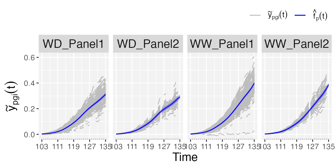

Plots at genotype level

At genotype level we can visualise three plots:

• If plotType = "popGenoTra", estimated population (\(\hat{f}_p(t)\)) and genotype-specific (\(\hat{f}_p(t)+\hat{f}_{pg}(t)\)) trajectories are depicted for all genotypes separately for each population. \(95\%\) pointwise confidence intervals are depicted for the estimated population trajectories.

  ## Population and genotype-specific trajectories.
  plot(pred.psHDM, plotType = "popGenoTra", themeSizeHDM = 10)

• If plotType = "popGenoDeriv", first-order derivative of the estimated population (\(\hat{f}'_p(t)\)) and genotype-specific (\(\hat{f}'_p(t)+\hat{f}'_{pg}(t)\)) trajectories are depicted for all genotypes separately for each population. \(95\%\) pointwise confidence intervals are depicted for estimated trajectories at the population level.

  ## First-order derivative of the population- and genotype-specific trajectories.
  plot(pred.psHDM, plotType = "popGenoDeriv", themeSizeHDM = 10)

• Finally, if plotType = "GenoDev", estimated genotype-specific deviations (\(\hat{f}_{pg}(t)\)) are depicted for all genotypes separately for each population.
  

  ## Genotype-specific deviations.
  plot(pred.psHDM, plotType = "genoDev", themeSizeHDM = 10)

Plots at plot level

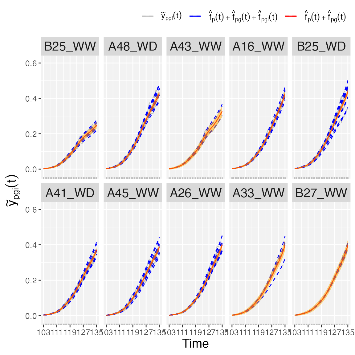
Finally, if we are interested in obtaining plots at the plot level, we use plotType = "genoPlotTra". Here, estimated genotype (\(\hat{f}_p(t)+\hat{f}_{pg}(t)\)) and plot-specific (\(\hat{f}_p(t)+\hat{f}_{pg}(t)+\hat{f}_{pgi}(t)\)) trajectories are depicted for all plots separately for a selection of genotypes. Also, \(95\%\) pointwise confidence intervals are depicted for the estimated genotype-specific trajectories. For this plotType, the user has the option to change names (genotypeNames) and/or order (genotypeOrder) of the selected genotypes.

## As an example we used ten randomly selected genotypes 
set.seed(1)
plot.genos  <- sample(pred.psHDM$genoLevel$genotype,10, replace = FALSE)
names.genos <- substring(plot.genos, first = 5)
names.genos
#>  [1] "B25_WW" "A48_WD" "A43_WW" "A16_WW" "B25_WD" "A41_WD" "A45_WW" "A26_WW"
#>  [9] "A33_WW" "B27_WW"

## Genotype- and plot-specific trajectories.
plot(pred.psHDM, 
     plotType = "genoPlotTra", 
     genotypes = plot.genos, genotypeNames = names.genos,
     themeSizeHDM = 10)

---

References

Pérez-Valencia, Diana M, María Xosé Rodríguez-Álvarez, Martin P Boer, Lukas Kronenberg, Andreas Hund, Llorenç Cabrera-Bosquet, Emilie J Millet, and Fred A van Eeuwijk. 2022. “A Two-Stage Approach for the Spatio-Temporal Analysis of High-Throughput Phenotyping Data.” Scientific Reports 12 (1): 1–16. https://doi.org/10.1038/s41598-022-06935-9.

Rodríguez-Álvarez, María, Martin P. Boer, Fred van Eeuwijk, and Paul H. C. Eilers. 2018. “Correcting for Spatial Heterogeneity in Plant Breeding Experiments with P-Splines.” Spatial Statistics 23 (October): 52–71. https://doi.org/10.1016/j.spasta.2017.10.003.

Wood, Simon N, Fabian Scheipl, and Julian J Faraway. 2013. “Straightforward Intermediate Rank Tensor Product Smoothing in Mixed Models.” Statistics and Computing 23 (3): 341–60. https://doi.org/10.1007/s11222-012-9314-z.