Calculate stability coefficients for genotype-by-environment data

This function calculates different measures of stability, the cultivar-superiority measure of Lin & Binns (1988), Shukla's (1972) stability variance and Wricke's (1962) ecovalence.

Usage

gxeStability(
  TD,
  trials = names(TD),
  trait,
  method = c("superiority", "static", "wricke"),
  bestMethod = c("max", "min"),
  sorted = c("descending", "ascending", "none")
)

Arguments

TD: An object of class TD.
trials: A character string specifying the trials to be analyzed. If not supplied, all trials are used in the analysis.
trait: A character string specifying the trait to be analyzed.
method: A character vector specifying the measures of stability to be calculated. Options are "superiority" (cultivar-superiority measure), "static" (Shukla's stability variance) or "wricke" (wricke's ecovalence).
bestMethod: A character string specifying the criterion to define the best genotype. Either "max" or "min".
sorted: A character string specifying the sorting order of the results.

Value

An object of class stability, a list containing:

superiority: A data.frame containing values for the cultivar-superiority measure of Lin and Binns.
static: A data.frame containing values for Shukla's stability variance.
wricke: A data.frame containing values for Wricke's ecovalence.
trait: A character string indicating the trait that has been analyzed.

References

Lin, C. S. and Binns, M. R. 1988. A superiority measure of cultivar performance for cultivar x location data. Can. J. Plant Sci. 68: 193-198

Shukla, G.K. 1972. Some statistical aspects of partitioning genotype-environmental components of variability. Heredity 29:237-245

Wricke, G. Uber eine method zur erfassung der okologischen streubreit in feldversuchen. Zeitschrift für Pflanzenzucht, v. 47, p. 92-96, 1962

Examples

## Compute three stability measures for TDMaize.
geStab <- gxeStability(TD = TDMaize, trait = "yld")

## Summarize results.
summary(geStab)
#> 
#> Cultivar-superiority measure (Top 10 % genotypes)
#>  Genotype     Mean Superiority
#>      G118 226.8275    213285.9
#>      G076 251.9900    188640.3
#>      G113 248.1250    185923.6
#>      G140 268.2125    181521.7
#>      G180 273.3250    179532.3
#>      G073 275.3838    173008.6
#>      G133 311.3375    165407.6
#>      G112 321.4125    156828.7
#>      G041 367.7250    153098.9
#>      G008 326.6000    152794.6
#>      G017 310.5500    149955.2
#>      G090 316.5625    147096.2
#>      G021 321.4625    147089.7
#>      G004 321.4250    145401.7
#>      G143 327.2750    142009.5
#>      G139 335.4875    140698.0
#>      G111 341.4250    139488.0
#>      G126 344.0288    139351.6
#>      G038 331.5750    139067.9
#>      G095 334.0500    137072.9
#>      G174 344.5500    136538.3
#>      G211 349.0625    135962.9
#> 
#> Static stability (Top 10 % genotypes)
#>  Genotype     Mean   Static
#>      G042 561.3875 185082.7
#>      G091 510.4500 184739.4
#>      G194 521.4250 180439.8
#>      G055 616.8500 180228.1
#>      G061 585.7500 179620.2
#>      G103 510.8000 175153.7
#>      G130 601.4000 163529.5
#>      G192 676.1375 163323.5
#>      G028 663.5625 159318.6
#>      G037 489.1250 158294.3
#>      G145 490.1750 157766.5
#>      G172 553.3750 156891.8
#>      G047 448.2125 156613.1
#>      G009 435.2000 154190.1
#>      G105 522.5500 152883.7
#>      G019 743.8250 152822.0
#>      G150 415.9125 151083.5
#>      G168 584.1000 149636.8
#>      G025 573.1375 149223.8
#>      G082 539.0750 149223.6
#>      G110 503.7375 147909.1
#>      G117 449.1000 146968.8
#> 
#> Wricke's ecovalence (Top 10 % genotypes)
#>  Genotype     Mean   Wricke
#>      G041 367.7250 421753.2
#>      G028 663.5625 225014.0
#>      G042 561.3875 207410.2
#>      G133 311.3375 199560.4
#>      G176 440.2000 187066.1
#>      G061 585.7500 186751.7
#>      G118 226.8275 183468.1
#>      G009 435.2000 182984.1
#>      G198 561.0750 182165.8
#>      G114 468.2500 179699.9
#>      G172 553.3750 174196.6
#>      G045 606.2000 173102.0
#>      G117 449.1000 172092.7
#>      G008 326.6000 170986.0
#>      G047 448.2125 170352.2
#>      G112 321.4125 168838.3
#>      G128 397.6375 157048.9
#>      G091 510.4500 155332.5
#>      G032 523.1375 152330.9
#>      G077 560.8250 151845.0
#>      G055 616.8500 150406.8
#>      G086 452.3000 150102.7

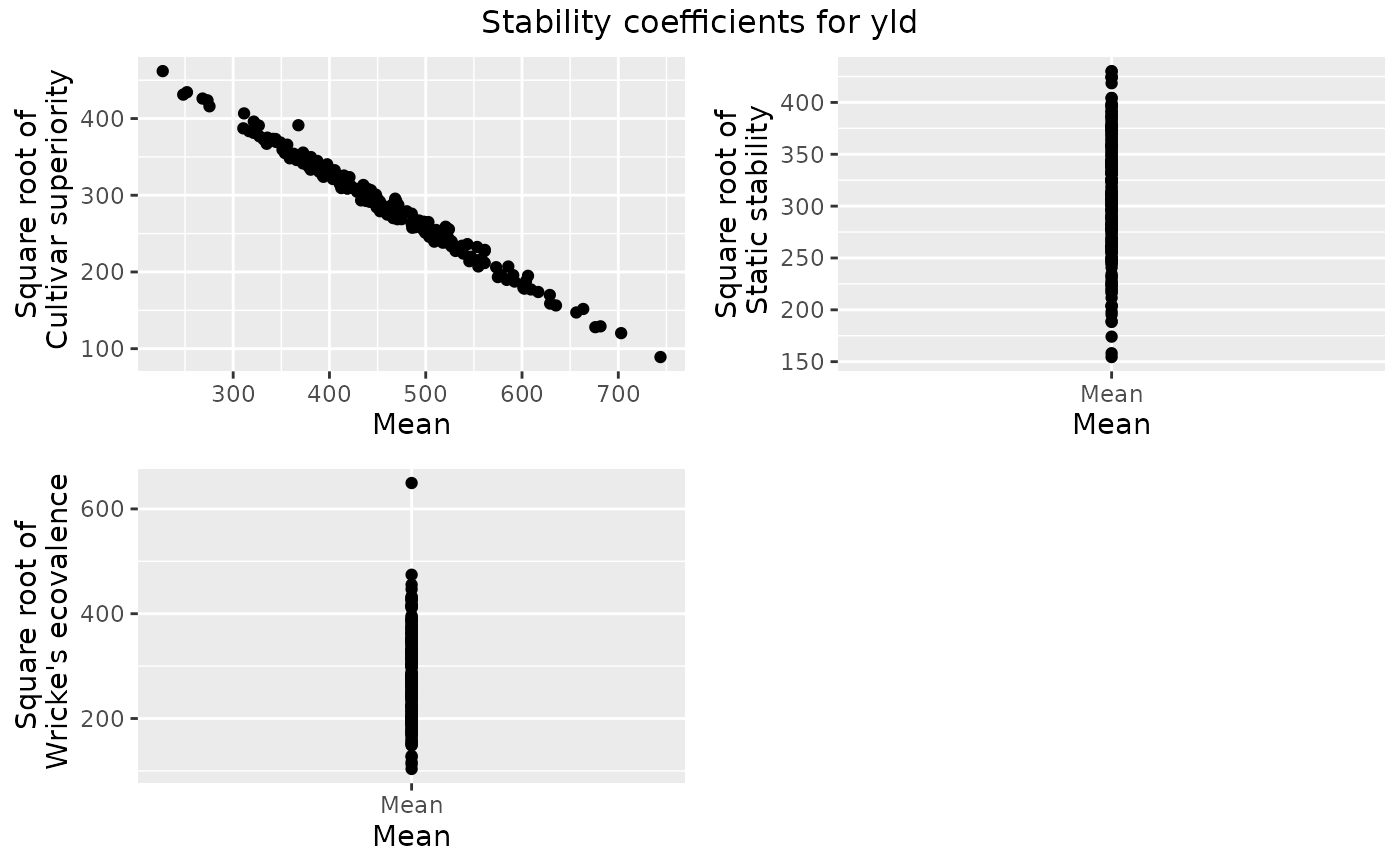
## Create plot of the computed stability measures against the means.
plot(geStab)


# \donttest{
## Create a .pdf report summarizing the stability measures.
report(geStab, outfile = tempfile(fileext = ".pdf"))
#> Error in report.stability(geStab, outfile = tempfile(fileext = ".pdf")): An installation of LaTeX is required to create a pdf report.
# }

## Compute Wricke's ecovalance for TDMaize with minimal values for yield as
## the best values. Sort results in ascending order.
geStab2 <- gxeStability(TD = TDMaize, trait = "yld", method = "wricke",
                       bestMethod = "min", sorted = "ascending")
summary(geStab2)
#> 
#> Wricke's ecovalence (Top 10 % genotypes)
#>  Genotype     Mean   Wricke
#>      G163 412.3125 10758.99
#>      G190 470.6250 12696.93
#>      G031 452.5750 13639.19
#>      G138 358.8750 15972.32
#>      G011 393.5125 16547.87
#>      G049 434.9625 22109.51
#>      G196 435.7000 22397.20
#>      G040 393.7750 23161.62
#>      G066 508.8500 23535.07
#>      G173 358.7250 23986.23
#>      G022 432.9000 25195.53
#>      G057 466.2875 25888.58
#>      G132 438.5000 27982.65
#>      G003 474.9250 28050.84
#>      G164 485.9625 29212.43
#>      G052 449.0000 29389.23
#>      G098 383.3625 29967.63
#>      G188 380.5125 30302.95
#>      G072 499.4875 30894.87
#>      G070 410.7875 31783.30
#>      G063 436.0875 32108.69
#>      G015 353.7750 33050.07